Post-Processing (Applying Survey Biases)

How it Works

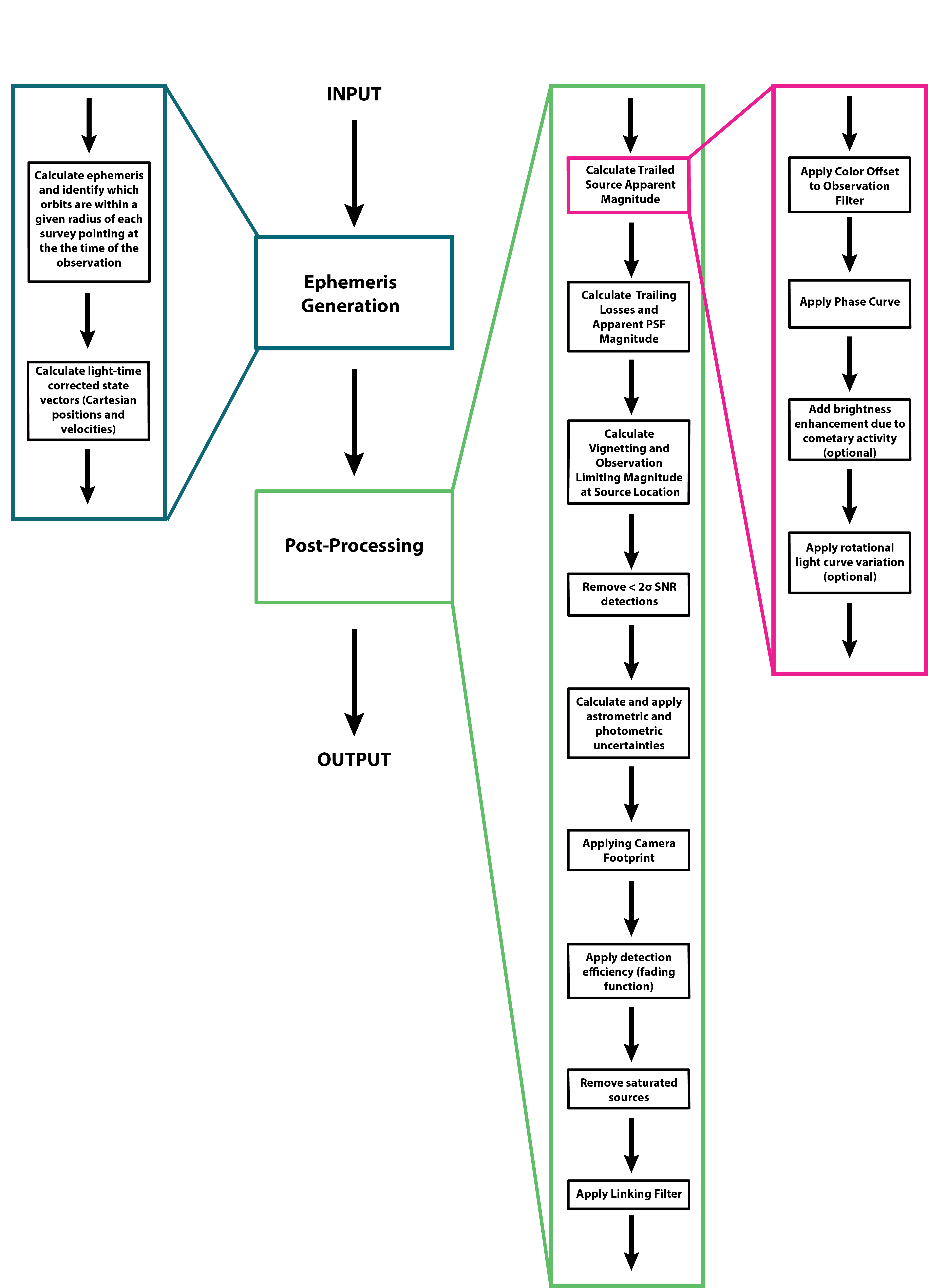
Once the ephemerides have been generated or read in from an external file, Sorcha moves on to the second phase, which we call post-processing. For each of the input objects, Sorcha goes through the potential detections identified in the ephemeris generation step and performs a series of calculations and assessments in the post-processing stage to determine whether the objects would have been detectable as a source in the survey images and would have later been identified as a moving solar system object. All aspects of post-processing can be adjusted or turned on/off via Sorcha's Configuration File.

See also

For a more detailed description of Sorcha's post-processing stage please see Merritt et al. (submitted).

The steps within Sorcha's post-processing stage that are used to estimate what the LSST would discover are shown below.

Calculating the Trailed Source Magnitude and PSF (Point Spread Function) Magnitude

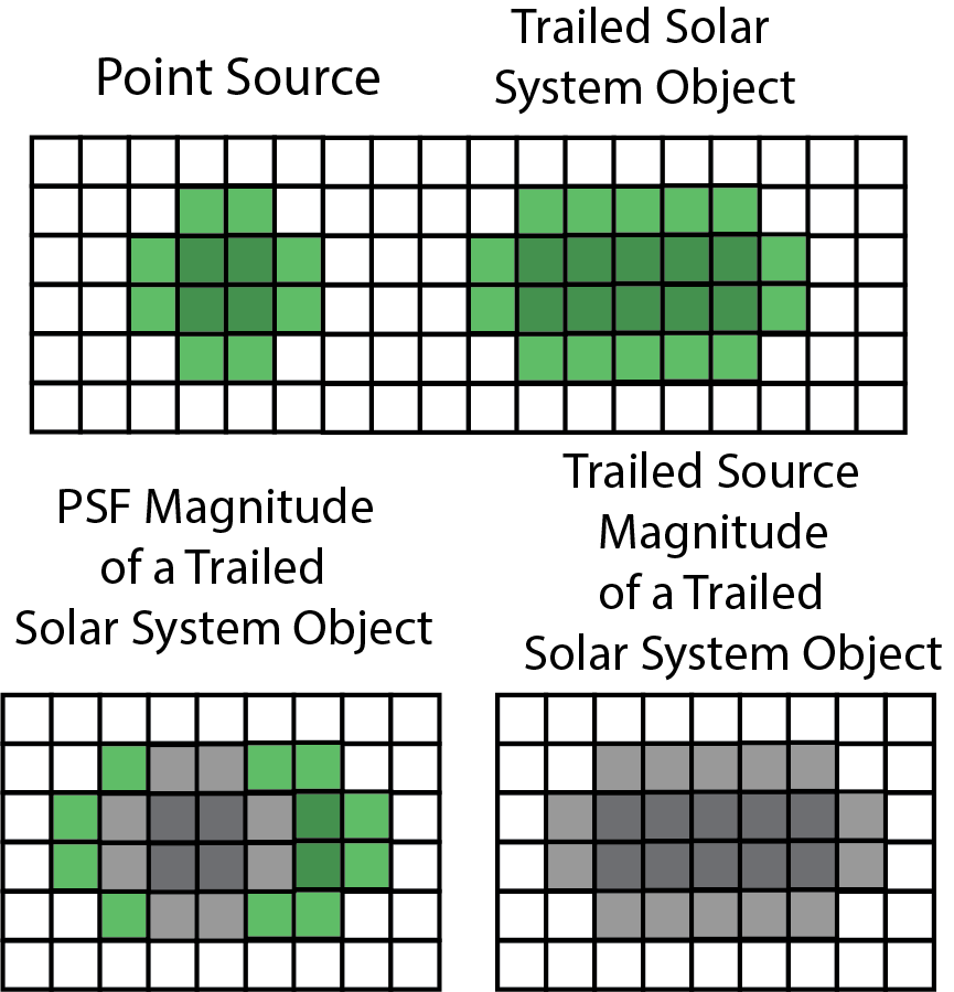
Sorcha calculates two apparent magnitudes that we will refer to as the trailed source magnitude and the PSF magnitude.

Unlike background stars, a moving solar system object may leave a streak on the detector, depending on the object’s on-sky velocity, the image exposure time, the camera’s pixel resolution, and the image quality, resulting in an extended PSF (“trail”) spanning more pixels than a point source would. The trailed source magnitude is the true apparent magnitude of the object (and the apparent magnitude that will be eventually calculated by the Rubin Solar System Processing pipelines), whereas the PSF magnitude (discussed is the effective brightness of the solar system object measured by the Rubin source detection algorithm (Difference Image Analysis; DIA). The PSF magnitude accounts for the loss in SNR (signal-to-noise ratio) from the flux being spread out over more pixels than a stellar profile would and the loss in flux from the Rubin source detection algorithms which use stellar PSF-like matched filter to identify transient sources in the survey’s difference images.

Sorcha first calculates the trailed source magnitude and later will calculate the PSF magnitude. Below is a cartoon schematic depicting the difference between how the trailed source magnitude and the PSF magnitude for a moving solar system object observed on an LSST image are estimated by the Rubin data management pipelines (including Solar System Processing [SSP]). The Rubin Data Management source detection pipeline, the Difference Image Analysis (DIA) pipeline, uses PSF filter matching to find sources on the image. This pipeline will measure the PSF magnitude. Only transient sources identified by the DIA pipeline will be sent on to the Rubin Solar System Processing (SSP) pipelines to search for moving objects. The SSP pipelines will report the trailed source magnitude.

A cartoon explanation of trailed source mag and PSF mag

For the LSST and its expected∼30 s exposures, objects whose rates of motion are 0.16 deg/day will trail 0.2′′, the size of a LSSTCam pixel. With a median expected seeing of 0.7′′≈3.5 pixels, we then expect that objects with rates of motion ≳ 0.4 deg/day, such as the closest MBAs (main-belf asteroids) and NEOs (Near-Earth objects), will have trails roughly comparable to half their PSF full at width at half maximum (FWHM), whereas the most distant objects (e.g. TNOs [Trans-Neptunian Objects]) will mostly appear as point sources. The longer the trail, the larger the difference between the trailed source magnitude and the PSF magnitude. For TNOs and more distant objects, the PSF magnitude and the trailed source magnitude will be nearly identical because of their slow rates.

Warning

When analyzing the detections and discoveries output from a Sorcha simulation, we caution the user to only use the trailed source magnitude. Using the PSF magnitude will give incorrect results because it is missing some of the object’s flux. The PSF magnitude is only used to assess detectability/apply the survey detection efficiency.

Colors and Phase Curves

For each potential detection of an object from the input population, the trailed source magnitude is calculated for the relevant observing filter using the colors specificed in the Physical Parameters File. The trailed source magnitude is also adjusted for phase curve effects. We have implemented several phase curve parameterizations that can be specified in the configuration file and then inputted through the Physical Parameters File. You can either specify one set of phase curve parameters for all observing filters or specify values for each observing filter examined by Sorcha. We are using the sbpy phase function utilities. The supported options are:

HG
HG1G2
HG12
linear (specified by S in the header of the Physical Parameters File)
none (if no columns for phase curve are included in the physical parameters file then the synthetic object is considered to have a flat phase curve).

Note

The HG12 model is the Penttilä et al. (2016) modified model, and not the original (IAU adopted) Muinonen et al. (2010) model.

The phase curve function to apply is set via the [PHASECURVES] section of the Configuration File

[PHASECURVES]

# The phase function used to calculate apparent magnitude. The physical parameters input
# file must contain the columns needed to calculate the phase function.
# Options: HG, HG1G2, HG12, linear, none.

phase_function = HG12

Accounting for Cometary Activity and Rotational Light Curves

Sorcha has the capability of accounting for the rotational light curve and cometary activity effects on the calculated trailed source magnitude. Further details are available in the Incorporating Rotational Lightcurves and Cometary Activity section.

Applying Trailing Losses and Calculating the PSF Magnitude

Once Sorcha calculates the trailed source magnitude for all potential detections, it then calculates the PSF magnitude for each potential detection accounting for trailing losses (the effect that the simulated moving object does not have a perfect point-source PSF but is instead elongated due the object's on-sky motion). Simulated moving object is moving fast enough in the potential detection's observation, the flux would form a trail (elongated source on the image in the direction of the object's motion), changing the apparent magnitude that the survey's source detection software will measure as well as decrease the SNR of the trailed source magnitude compared to a point source. Sorcha's trailing loss functions calculates these trailing losses to be used by the rest of the post-processing stage.

In order to estimate the astrometric and photometric uncertainties and determine the PSF magnitude, sorcha calculates for each potential detection the equivalent photometric losses caused by the elongated PSFs. sorcha calculates these losses as magnitude offsets to the trailed source magnitude. Sorcha uses the trailing loss implementation developed by Jones et al. (2018) and their best-fit values for the parametrizations estimated for the LSST.

There are two different trailing losses that must be calculated. The first is the trailing loss due to the smearing of the photometric signal over a larger number of pixels than for a point-source PSF, $\Delta m(\textrm{PSF})$, the PSF trailing loss. The second is the trailing loss due to the Rubin Data Management software detection algorithm attempting to identify sources on the image using a stellar PSF-like matched filter. We refer to this as the detection trailing loss, $\Delta m(\textrm{PSF + detection})$, as it accounts for both the matched filter excluding part of the trail and the SNR losses due to the object's flux being distributed differently than a point source for the pixels that are included by the detection algorithm.

The PSF magnitude ($m_{\textrm{PSF}}$) and the trailed source magnitude ($m_{\textrm{trailed source}}$) are related by:

\[m_{\textrm{PSF}} = m_{\textrm{trailed source}}+\Delta m(\textrm{PSF + detection})\]

The PSF trailing loss will be used later to calculate the uncertainty of the trailed source magnitude as $m_{\textrm{trailed source}}+\Delta m(\textrm{PSF})$ provides the apparent magnitude of a point-source with the equivalent SNR as what would be measured for the trailed PSF.

Sky image showing a short trailing source circled in red.

Left and Right: The trailing losses for different values of the seeing θ, shown as a function of the object’s on-sky velocity v, given in degrees per day on the bottom axis and pixels per 30 s visit on the upper axis. Right: A zoomed in version of the figure on the left for low v. Vertical lines represent the thresholds for typical on-sky motions of a TNO (Trans-Neptunian object), a Jupiter Trojan, and inner and outer MBAs (main-belt asteroids), a Jupiter Trojan, and inner and outer MBAs (main-belt asteroids) (Luu & Jewitt 1988, Equation 1).

Warning

Right now Sorcha only has functions to compute the trailing losses for the LSST.

Applying Photometric and Astrometric Uncertainties and Randomization

Real astronomical surveys measure photometry and astrometry that have uncertainties. To better compare to what the survey detected, for each potential detection of the input small body population, Sorcha applies photometric and astrometric errors that modify the calculated values for the right ascension, declination, trailed source magnitude, and PSF masgnitude. Sorcha computes the uncertainties for each potential detection of the input population and use them to characterize a normal distribution with a mean equal to the true value. Full details are provided in Merritt et al. (submitted).

Note

As a compromise between low-probability detections and unrealistic magnitude uncertainties producing “fake detections”, by default Sorcha removes all observations with the trailed source magnitude SNR is less than 2 after calculating the astrometric and photometric uncertainties.

Warning

Right now Sorcha only has functions to compute the photometric and astrometric uncertainties and SNR estimations specifically for Rubin Observatory.

See also

We have a Jupyter notebook demonstrating the application of the uncertainties and randomization of the photometric and astrometric values within Sorcha.

Validating Sorcha's Trailed Source Magnitude Calculations

See also

See our Jupyter notebook that validates the apparent magnitude calculation.

Incorporating Rotational Lightcurves and Cometary Activity

Sorcha has the ability user provided functions though python classes that augment/change the apparent brightness calculations for the synthetic Solar System objects. Any values required as input for these calculations, must be provided in the separate Complex Physical Parameters File (Optional) file as input. Rather than forcing the user directly modify the Sorcha codebase every time they want to apply a different model for representing the effects of rotational light curves or cometary activity, we provide the ability to develop separate activity and light curve/brightness enhancement functions as plugins using our template classes and add them to the Sorcha add-ons package. In both cases, any derived class must inherit from the corresponding base class and follow its API, to ensure that Sorcha knows how to find and use your class. Once the Sorcha add-ons is installed, Sorcha will automatically detect the available plugins and make them available during post-processing. To use one of the plugins from the community utilities, simply add the unique name of the plugin to the Configuration File provided to Sorcha, and provide the Complex Physical Parameters File (Optional) file on the command line. We currently have 2 pre-made classes that can augment the calculated apparent magnitude of each synthetic object, One for handling cometary activity as a function of heliocentric distance and one that applies rotational light curves to the synthetic objects.

Cometary Activity or Simulating Other Active Objects

A user can use the cometary activity prescriptions available in the Sorcha add-ons package or add their own class to apply a different cometary activity model in a custom version of the Sorcha add-ons package. Once the Sorcha add-ons package is installed, Sorcha will automatically detect the available plugins and make them available during processing.

Cometary Activity Configuration Parameters

Set the cometary_activity configuration file file variable to none if you do you want to apply any cometary activity brightness enhancements to Sorcha's apparent magnitude calculations.

[ACTIVITY]

# The unique name of the actvity model to use. Defined in the ``name_id`` method
#  of the subclasses of AbstractCometaryActivity.  If not none, a complex physical parameters
# file must be specified at the command line.

comet_activity = lsst_comet

Tip

To not include an cometary activity effects on the apparent magnitude calculations, set comet_activity to none.

Cometary Activity Template Class

from abc import ABC, abstractmethod
from typing import List
import logging
import pandas as pd
import numpy as np

logger = logging.getLogger(__name__)


class AbstractCometaryActivity(ABC):
    """Abstract base class for cometary activity models"""

    def __init__(self, required_column_names: List[str] = []) -> None:
        """Abstract base class accepts a list of column names that are required
        to be present in the Pandas dataframe passed to the ``compute`` method.

        Parameters
        ----------
        required_column_names : list, optional
            The list of columns in ``observations`` dataframe that are required
            for the model calculation, by default []
        """
        self.required_column_names = required_column_names

    @abstractmethod
    def compute(self, df: pd.DataFrame) -> np.array:
        """User implemented calculation based on the input provided by the
        pandas dataframe ``df``.

        Parameters
        ----------
        df : Pandas dataframe
            The ``observations`` dataframe provided by ``Sorcha``.
        """
        raise NotImplementedError("Must be implemented by the subclass")

    def _validate_column_names(self, df: pd.DataFrame) -> None:
        """Private method that checks that the provided pandas dataframe contains
           the required columns defined in ``self.required_column_names``.

        Parameters
        ----------
        df : Pandas dataframe
            The ``observations`` dataframe provided by ``Sorcha``.
        """
        for colname in self.required_column_names:
            if colname not in df.columns:
                err_msg = f"Input dataframe is missing column %{colname}"
                self._log_error_message(error_msg=err_msg)
                raise ValueError(err_msg)

    def _log_exception(self, exception: Exception) -> None:
        """Log an error message from an exception to the error log file

        Parameters
        ----------
        exception : Exception
            The exception with a value string to appended to the error log
        """
        self._log_error_message(str(exception.value))

    def _log_error_message(self, error_msg: str) -> None:
        """Log a specific error string to the error log file

        Parameters
        ----------
        error_msg : str
            The string to be appended to the error log
        """
        logger.error(error_msg)

    @staticmethod
    @abstractmethod
    def name_id() -> str:
        """This method will return the unique name of the LightCurve Model"""
        raise NotImplementedError("Must be implemented as a static method by the subclass")

LSSTCometActivity Class

Inside the Sorcha add-ons GitHub repository, we provide an example of a comet activity class. To use this function, in the Complex Physical Parameters File (Optional) file, the user must provide a dust falling exponential value (k), the ${af\rho}$, the product of albedo, the filling factor of grains within the observer field of view, and the linear radius of the field of view (typically selected to be 10,000 km) for the comet when it is located at a heliocentric distance of 1 au (${af\rho_{1}}$), Observing filter of the observation (optFilter), Apparent magnitude in the input filter of the comet nucleus adding up all of the counts in the trail (TrailedSourceMag). If these are not provided then the software will produce an error message. We have an example Jupyter notebook demonstrating the LSSTCometActivity class built into Sorcha add-ons package. To use this prescription the comet_activity configuration file variable should be set to lsst_comet. The ${af\rho(r)}$ at the given observation is then estimated using the equation

\[af\rho(r) = af\rho_{1} \cdot r^{k} \cdot f(\alpha)\]

Where ${f(\alpha)}$ is the Halley-Marcus phase function at phase angle ({alpha}) from Schleicher.

Rotational Lightcurve Effects

Rotational Light Curve Configuration Parameters

A user can use the rotational light curve prescriptions available in the Sorcha add-ons package or add their own class to apply a different model for rotation effects in a custom version of the Sorcha add-ons package. Once the Sorcha add-ons package is installed, Sorcha will automatically detect the available plugins and make them available during processing.

[LIGHTCURVE]


# The unique name of the lightcurve model to use. Defined in the ``name_id`` method
# of the subclasses of AbstractLightCurve. If not none, the complex physical parameters
# file must be specified at the command line.lc_model = none

lc_model = none

Set the lc_model configuration file varialble to none if you do you want to apply any light curve effects to Sorcha's apparent magnitude calculations.

Lightcurve Template Class

from abc import ABC, abstractmethod
from typing import List
import logging
import numpy as np
import pandas as pd

logger = logging.getLogger(__name__)


class AbstractLightCurve(ABC):
    """Abstract base class for lightcurve models"""

    def __init__(self, required_column_names: List[str] = []) -> None:
        """Abstract base class accepts a list of column names that are required
        to be present in the Pandas dataframe passed to the ``compute`` method.

        Parameters
        ----------
        required_column_names : list, optional
            The list of columns in ``observations`` dataframe that are required
            for the model calculation, by default []
        """
        self.required_column_names = required_column_names

    @abstractmethod
    def compute(self, df: pd.DataFrame) -> np.array:
        """User implemented calculation based on the input provided by the
        pandas dataframe ``df``.

        Parameters
        ----------
        df : Pandas dataframe
            The ``observations`` dataframe provided by ``Sorcha``.
        """
        raise NotImplementedError("Must be implemented by the subclass")

    def _validate_column_names(self, df: pd.DataFrame) -> None:
        """Private method that checks that the provided pandas dataframe contains
           the required columns defined in ``self.required_column_names``.

        Parameters
        ----------
        df : Pandas dataframe
            The ``observations`` dataframe provided by ``Sorcha``.
        """
        for colname in self.required_column_names:
            if colname not in df.columns:
                err_msg = f"Input dataframe is missing column %{colname}"
                self._log_error_message(error_msg=err_msg)
                raise ValueError(err_msg)

    def _log_exception(self, exception: Exception) -> None:
        """Log an error message from an exception to the error log file

        Parameters
        ----------
        exception : Exception
            The exception with a string to appended to the error log
        """
        self._log_error_message(str(exception))

    def _log_error_message(self, error_msg: str) -> None:
        """Log a specific error string to the error log file

        Parameters
        ----------
        error_msg : string
            The string to be appended to the error log
        """
        logger.error(error_msg)

    @staticmethod
    @abstractmethod
    def name_id() -> str:
        """This method will return the unique name of the LightCurve Model"""
        raise NotImplementedError("Must be implemented as a static method by the subclass")

Sinusoidal Light Curve Class

Inside the Sorcha add-ons GitHub repository, we provide a simple example implementation where the apparent magnitude of the object (that is, the magnitude after all geometric effects have been taken into account), has a sinusoidal term added to it. To use this function, in the Complex Physical Parameters File (Optional) file, the user must provide a light curve amplitude (LCA), corresponding to half the peak-to-peak amplitude for the magnitude changes, a period Period, and a reference time Time0 where the light curve is at 0 - if these are not provided, the software will produce an error message. Despite being simple, that implementation shows all the class methods that need to be implemented for a custom light curve function. We have an example Jupyter notebook demonstrating the SinusoidalLightCurve class built into Sorcha add-ons package, To use this prescription, the lc_model configuration file variable should be set to sinusoidal.

Calculating the 5σ Limiting Magnitude at the Source Location and Vignetting

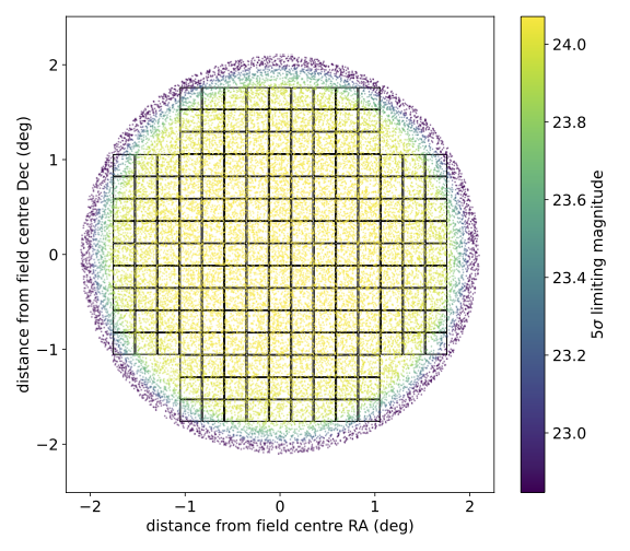
Objects that are on the edges of the field of view are dimmer due to vignetting: the field-of-view is not uniformly illuminated, and so the limiting magnitude for each detection will depend on its position within the FOV (field-of-view). The effect of this is to decrease the 5σ limiting magnitude – the apparent magnitude where a detected point source has exactly a 50% probability of detection – at the edges of the LSSTCam FOV. Sorcha accommodates this by calculating the effects of vignetting at the source’s location on the focal plane and adjusting the 5σ limiting magnitude accordingly for each potential detection. This modified limiting magnitude will be used when applying the survey detection efficiency. We call this value the 5σ Limiting Magnitude at the Source Location ($m_{5\sigma}$).

Sorcha applies a vignetting model from a built-in function tailored specifically for the LSST (see Araujo-Hauck et al. 2016). The image below shows the effects of vignetting on the 5σ limiting magnitude for a randomized series of points on a circular FOV in the LSSTCam focal plane. The LSSTCam detector footprint is also plotted. Locations further from the center of the FOV have shallower depths.

Plot of the LSST camera footprint in Dec vs. RA, showing shaded dimming due to vignetting.

Note

The Survey Pointing Database provides the 5σ limiting magnitude at the center of the exposure's FOV.

Note

Sorcha currently only has a vignetting model for the LSSTCam.

See also

We have a Jupyter notebook demonstrating Sorcha's vignetting calculation.

Applying the Camera Footprint Filter

Due to the footprint of the LSST Camera (LSSTCam), see the figure below, it is possible that some object detections may be lost in gaps between the chips.

Plot of the LSST camera footprint where x and y are x and y distance from the pupil in degrees. The footprint also shows two overplotted circle radii of 1.75deg (corresponding to a 75% fill factor) and 2.06deg.

However, the full camera footprint is most relevant for slow-moving objects, where an object may move only a small amount per night and could thus in a subsequent observation fall into a chip gap. This is less concerning for faster-moving objects such as asteroids and near-Earth objects. As a result, we provide two methods of applying the camera footprint.

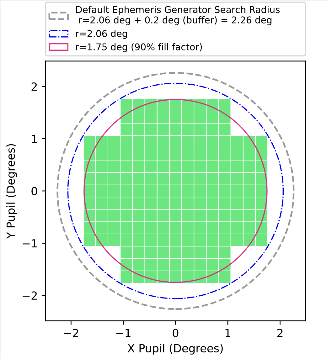
Circle Radius (Simple Sensor Area)

Using this filter applies a very simple circular camera footprint. The radius of the circle (circle_radius key) should be given in degrees. The fill_factor key specifics what fraction of observations should be randomly removed to roughly mimic detector chip gaps in this circular footprint approximation. The fraction of observations not removed is controlled by the config variable fill_factor. To include this filter, the following options should be set in the Configuration File:

[FOV]
camera_model = circle
circle_radius = 1.75
fill_factor = 0.9

Warning

Note that the internal ephemeris generator also uses a circular radius for its search area. To get accurate results, the ephemeris generator search radius must be set to be larger than the circle_radius. For simulating the LSST, we recommend setting ar_ang_fov = 2.06 and ar_fov_buffer = 0.2. Setting the circle_radius to be larger than the radius used for the ephemeris generation stage will have no effect.

Tip

Applying the fill factor in the circle radius camera filter is option. If the fill_factor is not present in the Configuration File then Sorcha includes all potential detections that land within the circular area.

Tip

For Rubin Observatory, the circle radius should be set to 1.75 degrees with a fill factor of 0.9 to approximate the detector area of LSSTCam.

See also

We have a Jupyter notebook demonstrating Sorcha's circle radius (simple sensor area) filter.

Full Camera Footprint

Using this filter applies a full camera footprint, including chip gaps. The full camera footprint filter figures out which of the possible input population detections (as identified by the ephemeris generation stage/input) for each survey observations land within on the survey camera's detectors. This is the slowest and most accurate version of the footprint filter. The image below shows the full camera footprint filter for the default LSSTCam architecture.

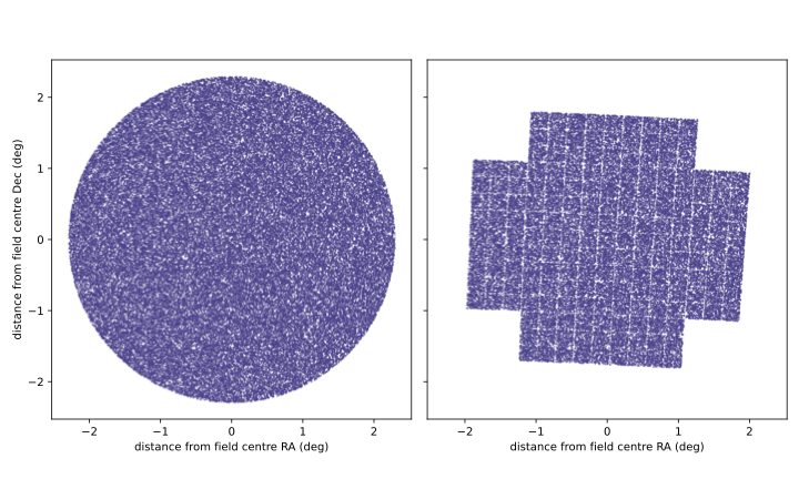
The effect of the full camera footprint filter on a selection of 100,000 random synthetic sources. Left: original sources, distributed over a circular FOV (field-of-view) of radius 2.1 degrees. Right: the same sources after running Sorcha’s full camera footprint filter. The shape of the LSSTCam detector footprint can be seen with the loss of detections in the raft and chip gaps.

To use the full camera footprint filter, the following option should be set in the Configuration File:

[FOV]
camera_model = footprint

Sorcha comes with a representation of the LSSTCam footprint already installed. If you do not include the footprint_path in the Configuration File, then Sorcha assumes you're using its internal LSSTCam footprint. Further details about supplying your own camera footprint file can be found in the Inputs page.

Warning

Note that the internal ephemeris generator uses a circular radius for its search area. To get accurate results, the ephemeris generation search radius must be set to be larger than the circle_radius. For simulating the LSST, we recommend setting ar_ang_fov = 2.06 and ar_fov_buffer = 0.2.

Additionally, the camera footprint model can account for the losses at the edge of the CCDs where the detection software will not be able to pick out sources close to the edge. You can add an exclusion zone around each CCD measured in arcseconds (on the focal plane) using the footprint_edge_threshold key to the configuration file. An example setup in the Configuration File:

[FOV]
camera_model = footprint
footprint_edge_threshold = 0.0001

Note

If footprint_edge_threshold is not includeed, then Sorcha will assume all of the CCD detector area should be considered.

See also

We have a Jupyter notebook demonstrating Sorcha's full camera footprint filter.

Applying the Source Detection Efficiency (Fading Function) Filter

This filter serves to remove potential detections of the input small bodies which are too faint to be detected in the relevant survey observation. For an input small body with a PSF magnitude of $m_{PSF}$ and a given survey observation with $5\sigma$ limiting magnitude at the source location ($m_{5\sigma}$), Sorcha uses the detection efficiency (fading function) formulation of Veres and Chesley (2017) where:

\[\epsilon(m_{PSF}) = \frac{F}{1 + e^\frac{m_{PSF}-m_{5\sigma}}{w}}\]

This fading function is parameterized by the fading function width ($w$) and peak efficiency ($F$).

Note

Currently Sorcha applies the same fading function parameters ($w$ and $F$) to all the simulated survey observations.

Graph showing the fading function. Detection probability is plotted against magnitude - limiting magnitude, showing three smoothed step-functions centred on 0.0 on the x axis for three different widths.

The figure above shows the source detection efficiency (fading function) and how Sorcha applies it. The top plot shows the fading function representing the fraction of detected point sources as a function of $5\sigma$ limiting magnitude at the source location. The different lines represent the effect of the variation of the peak detection efficiency and the width parameter on the shape of the function. The $5\sigma$ limiting magnitude at the source location is marked in gray (m5σ=24.5). The bottom plot show histogram showing detection probability of 10,000 point sources passed through Sorcha’s fading function filter, with the actual calculated detection probability from the efficiency function overplotted as a solid line. Here, peak detection efficiency = 1.0, width parameter = 0.1, and m5σ=24.5 and the binsize is 0.04 mag.

In Sorcha's implementation, the detection efficiency $\epsilon(m_{PSF})$ is calculated at the PSF magnitude for each potential detection of an input synthetic small body and compared to a random number selected for each detection opportunity from a uniform distribution. Those potential detections whose drawn random number is less than or equal to $epsilon(m)$ will be deemed ``detected" as an astronomical source on the relevant survey observation/pointing and will continue to be passed on to later stages of post-processing.

To configure the fading function, the following variables should be set in the Configuration File:

[FADINGFUNCTION]
fading_function_width = 0.1
fading_function_peak_efficiency = 1.

Note

The default values are modeled on those from the Annis et al. (2014).

See also

We have a Jupyter notebook showing how Sorcha applies the survey detection efficiency (fading function).

Accounting for Saturation (Saturation/Bright Limit Filter)

The saturation/bright limit filter removes all potential detections of the input population that are brighter than the saturation limit of the survey. Ivezić et al. (2019) estimate that the saturation limit for the LSST will be ~16 in the r filter.

Sorcha includes functionality to specify either a single saturation limit, or a saturation limit in each filter. For the latter, limits must be given in a comma-separated list in the same order as the observing filters set in the configuration file

To include this filter, the Configuration File should contain:

[SATURATION]
bright_limit = 16.0

Or:

[SATURATION]
bright_limit = 16.0, 16.1, 16.2

Tip

The saturation filter is only applied if the configuration file has a SATURATION section.

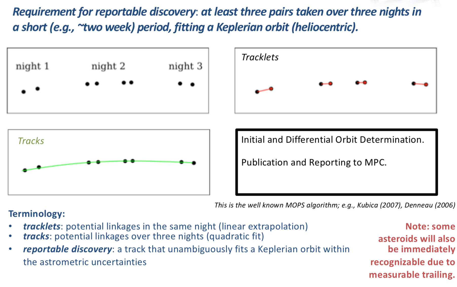
The Linking Filter

The linking filter simulates the behavior of LSST's Solar System Processing (SSP, Jurić et al. 2020, Swinbank et al. 2020), the automated software pipeline dedicated to linking and cross-matching observations that belong to the same object.

Linking is performed by detecting multiple observations of an object in a single night: a 'tracklet'. A number of these tracklets must then be detected in a specific time window to form a 'track'.

To use this filter, the user must specify all seven of the parameters in the Configuration File. The defaults given below are those used by SSP and are explained in the comments:

[LINKING]

# Not all objects will be linked by SSP: this variable controls the
# fraction successfully linked.
SSP_detection_efficiency = 0.95

# The number of observations required to form a valid tracklet.
SSP_number_observations = 2

# The minimum separation (in arcsec) between two observations of
# an object required for the linking to distinguish them as separate.
SSP_separation_threshold = 0.5

# The maximum time separation (in days) between subsequent
# observations in a tracklet.
SSP_maximum_time = 0.0625

# The number of tracklets required to form a track.
SSP_number_tracklets = 3

# Tracklets must occur in <= this number of days to constitute a
# complete track/detection.
SSP_track_window = 15

# The time in UTC at which it is noon at the observatory location (in standard time).
# For the LSST, 12pm Chile Standard Time is 4pm UTC.
SSP_night_start_utc = 16.0

Keeping Unlinked Objects

By default, when the linking filter is on unless otherwise specified Sorcha will drop all observations of unlinked objects. If the user wishes to retain these observations, this can be set in the Configuration File. This will add an additional column to the output, object_linked, which states whether the observation is of a linked object or not. To enable this functionality, add the following to the Configuration File:

[LINKING]
drop_unlinked = False

Note

If drop_unlinked is not present in the configuration file, Sorcha will go to its default setting of dropping all observations of unlinked objects. The Rubin Full Footprint and the Rubin Circular Approximation configuration file are set up this way.

See also

See our Jupyter notebook that validates the linking filter.

Tip

The linking filter is only applied if the configuration file has a LINKING section.

Specifying What Observations to Include

The user sets what observations from the survey Survey Pointing Database will be used by setting the observing_filters Configuration File variable in the [FILTERS] section:

[FILTERS]

# Filters of the observations you are interested in, comma-separated.
# Your physical parameters file must have H calculated in one of these filters
# and colour offset columns defined relative to that filter.

observing_filters = r,g,i,z,u,y

The first observing filters in the list are separated by a comma. The first observing filter listed should is the main filter that the absolute magnitude is defined for. The Physical Parameters File must have colors relative to the main filter specified for the input small body population.

If the user wants to use a subset of the observations, such as only including observations from the first year of the survey, the user can either modify the Survey Pointing Database or modify the Survey Pointing Database query in the Configuration File. We recommend the user modify the input survey pointing database in this situation.

Expert Advanced Post-Processing Features

Once a user is familiar with Sorcha and how it works, there are additional advanced post-processing tunable features and parameters available for the expert user.

Danger

With great power comes great responsibility. If you're new to Sorcha we strongly recommend that you first get familiar with running Sorcha and how it works before going on to apply any advanced post-processing features as they may produce unintended results. For many use cases, a user will likely not need to touch these parameters within Sorcha.

Attention

Applying some form of the camera footprint filter is mandatory if you are trying to preform a science quality simulation, but we do have the ability to turn it off for other types of modeling cases as an advanced post-processing tunable feature.