Apparent Magnitude Validation

import pandas as pd
import numpy as np
import astropy.units as u
from astroquery.jplhorizons import Horizons
from sorcha.modules.PPCalculateApparentMagnitudeInFilter import PPCalculateApparentMagnitudeInFilter
import matplotlib.pyplot as plt

To test the calculation of the apparent magnitude in the code, we can compare them to the apparent magnitudes calculated by JPL Horizons.

First, let’s get the JPL Horizons ephemeris for a test object. PPCalculateApparentMagnitudeInFilter uses sbpy’s photometry module to calculate phase functions, and sbpy’s unit tests use 24 Themis as a test object. We will do the same.

obj = Horizons(id='Themis', id_type='name', location='I11',

               epochs={'start':'2021-01-01', 'stop':'2023-01-01',

                       'step':'1d'})

eph = obj.ephemerides(quantities='9,19,20,43')
jpl_eph = eph.to_pandas()
jpl_eph

	targetname	datetime_str	datetime_jd	H	G	solar_presence	lunar_presence	V	surfbright	r	r_rate	delta	delta_rate	alpha_true	PABLon	PABLat
0	24 Themis (A853 GA)	2021-Jan-01 00:00	2459215.5	7.22	0.19	C		13.298	7.092	3.275241	1.868767	4.212453	-4.641369	4.5918	262.7496	-0.4684
1	24 Themis (A853 GA)	2021-Jan-02 00:00	2459216.5	7.22	0.19	C		13.307	7.102	3.276319	1.866016	4.209518	-4.922596	4.7832	263.0067	-0.4700
2	24 Themis (A853 GA)	2021-Jan-03 00:00	2459217.5	7.22	0.19	C		13.315	7.112	3.277396	1.863252	4.206423	-5.203712	4.9741	263.2635	-0.4716
3	24 Themis (A853 GA)	2021-Jan-04 00:00	2459218.5	7.22	0.19	C		13.324	7.122	3.278471	1.860476	4.203166	-5.484782	5.1645	263.5200	-0.4732
4	24 Themis (A853 GA)	2021-Jan-05 00:00	2459219.5	7.22	0.19	C		13.332	7.132	3.279545	1.857687	4.199749	-5.765845	5.3543	263.7760	-0.4748
...	...	...	...	...	...	...	...	...	...	...	...	...	...	...	...	...
726	24 Themis (A853 GA)	2022-Dec-28 00:00	2459941.5	7.22	0.19	C	m	13.460	7.606	3.407801	-1.337567	3.548593	23.738198	16.0868	357.7423	-0.3756
727	24 Themis (A853 GA)	2022-Dec-29 00:00	2459942.5	7.22	0.19	C	m	13.465	7.604	3.407028	-1.341288	3.562140	23.633204	16.0210	357.9249	-0.3731
728	24 Themis (A853 GA)	2022-Dec-30 00:00	2459943.5	7.22	0.19	C	m	13.471	7.601	3.406252	-1.345002	3.575623	23.523879	15.9522	358.1090	-0.3707
729	24 Themis (A853 GA)	2022-Dec-31 00:00	2459944.5	7.22	0.19	C	m	13.476	7.599	3.405474	-1.348708	3.589039	23.410433	15.8807	358.2945	-0.3683
730	24 Themis (A853 GA)	2023-Jan-01 00:00	2459945.5	7.22	0.19	C	m	13.481	7.596	3.404694	-1.352405	3.602385	23.293037	15.8063	358.4816	-0.3659

731 rows × 16 columns

This needs to be turned into a form the function can understand. Values for G1, G2 and G12 are from Muinonen et al. (2010).

observations_df = pd.DataFrame({'MJD':jpl_eph['datetime_jd'] - 2_400_000.5,
                                'H_filter': jpl_eph['H'],
                                'GS': jpl_eph['G'],
                                'G1': np.zeros(len(jpl_eph['G'])) + 0.62,
                                'G2': np.zeros(len(jpl_eph['G'])) + 0.14,
                                'G12': np.zeros(len(jpl_eph['G'])) + 0.68,
                                'JPL_mag': jpl_eph['V'],
                                'Range_LTC_km': jpl_eph['r'] * 1.495978707e8,
                                'Obj_Sun_LTC_km': jpl_eph['delta'] * 1.495978707e8,
                                'phase_deg': jpl_eph['alpha_true']})

observations_df

	MJD	H_filter	GS	G1	G2	G12	JPL_mag	Range_LTC_km	Obj_Sun_LTC_km	phase_deg
0	59215.0	7.22	0.19	0.62	0.14	0.68	13.298	4.899690e+08	6.301739e+08	4.5918
1	59216.0	7.22	0.19	0.62	0.14	0.68	13.307	4.901304e+08	6.297350e+08	4.7832
2	59217.0	7.22	0.19	0.62	0.14	0.68	13.315	4.902915e+08	6.292719e+08	4.9741
3	59218.0	7.22	0.19	0.62	0.14	0.68	13.324	4.904523e+08	6.287847e+08	5.1645
4	59219.0	7.22	0.19	0.62	0.14	0.68	13.332	4.906130e+08	6.282735e+08	5.3543
...	...	...	...	...	...	...	...	...	...	...
726	59941.0	7.22	0.19	0.62	0.14	0.68	13.460	5.097998e+08	5.308620e+08	16.0868
727	59942.0	7.22	0.19	0.62	0.14	0.68	13.465	5.096841e+08	5.328886e+08	16.0210
728	59943.0	7.22	0.19	0.62	0.14	0.68	13.471	5.095680e+08	5.349056e+08	15.9522
729	59944.0	7.22	0.19	0.62	0.14	0.68	13.476	5.094517e+08	5.369125e+08	15.8807
730	59945.0	7.22	0.19	0.62	0.14	0.68	13.481	5.093350e+08	5.389091e+08	15.8063

731 rows × 10 columns

Now we calculate the magnitude using the various models in PPCalculateApparentMagnitudeInFilter.

observations_df = PPCalculateApparentMagnitudeInFilter(observations_df.copy(), 'HG', 'r', 'HG_mag')
observations_df = PPCalculateApparentMagnitudeInFilter(observations_df.copy(), 'HG12', 'r', 'HG12_mag')
observations_df = PPCalculateApparentMagnitudeInFilter(observations_df.copy(), 'HG1G2', 'r', 'HG1G2_mag')

observations_df

	MJD	H_filter	GS	G1	G2	G12	JPL_mag	Range_LTC_km	Obj_Sun_LTC_km	phase_deg	HG_mag	HG12_mag	HG1G2_mag
0	59215.0	7.22	0.19	0.62	0.14	0.68	13.298	4.899690e+08	6.301739e+08	4.5918	13.311578	13.307267	13.296821
1	59216.0	7.22	0.19	0.62	0.14	0.68	13.307	4.901304e+08	6.297350e+08	4.7832	13.321366	13.316490	13.306087
2	59217.0	7.22	0.19	0.62	0.14	0.68	13.315	4.902915e+08	6.292719e+08	4.9741	13.330778	13.325410	13.315072
3	59218.0	7.22	0.19	0.62	0.14	0.68	13.324	4.904523e+08	6.287847e+08	5.1645	13.339831	13.334037	13.323783
4	59219.0	7.22	0.19	0.62	0.14	0.68	13.332	4.906130e+08	6.282735e+08	5.3543	13.348535	13.342378	13.332227
...	...	...	...	...	...	...	...	...	...	...	...	...	...
726	59941.0	7.22	0.19	0.62	0.14	0.68	13.460	5.097998e+08	5.308620e+08	16.0868	13.461646	13.498557	13.502578
727	59942.0	7.22	0.19	0.62	0.14	0.68	13.465	5.096841e+08	5.328886e+08	16.0210	13.467347	13.503931	13.507875
728	59943.0	7.22	0.19	0.62	0.14	0.68	13.471	5.095680e+08	5.349056e+08	15.9522	13.472879	13.509119	13.512982
729	59944.0	7.22	0.19	0.62	0.14	0.68	13.476	5.094517e+08	5.369125e+08	15.8807	13.478251	13.514132	13.517910
730	59945.0	7.22	0.19	0.62	0.14	0.68	13.481	5.093350e+08	5.389091e+08	15.8063	13.483454	13.518962	13.522651

731 rows × 13 columns

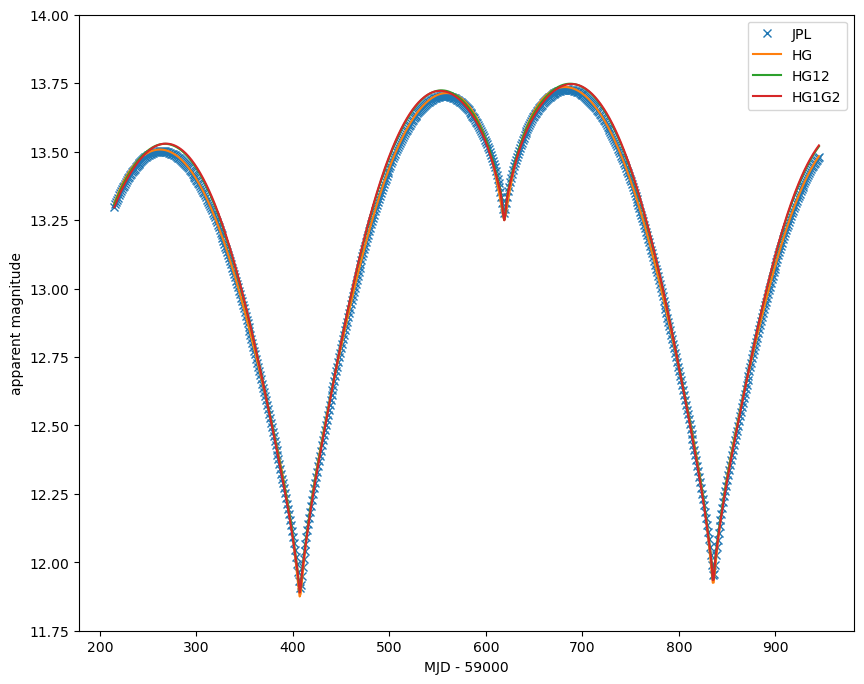
Now we can plot the magnitudes and compare them.

Note that we do not expect any of the calculated magnitudes to match JPL Horizons exactly. JPL Horizons uses the IAU simplification of the HG model to calculate apparent magnitude, while sbpy uses the original HG formulation from Bowell et al. (1989). However, they should all be a close match.

fig, ax = plt.subplots(figsize=(10,8))
ax.plot(observations_df["MJD"] - 59000, observations_df["JPL_mag"], linestyle="", marker="x", label="JPL")
ax.plot(observations_df["MJD"] - 59000, observations_df["HG_mag"], label="HG")
ax.plot(observations_df["MJD"] - 59000, observations_df["HG12_mag"], label="HG12")
ax.plot(observations_df["MJD"] - 59000, observations_df["HG1G2_mag"], label="HG1G2")
ax.legend()
ax.set_xlabel("MJD - 59000")
ax.set_ylabel("apparent magnitude")
ax.set_ylim((11.75, 14))
plt.show()

To test the linear phase function model, we simply define a slope. We will use the same values for Themis and arbitrarily choose S to be 0.04.

H = observations_df['H_filter'].values
alpha = observations_df['phase_deg'].values
r = observations_df['Range_LTC_km'].values / 1.495978707e8
delta = observations_df['Obj_Sun_LTC_km'].values / 1.495978707e8
S = np.zeros(len(H)) + 0.04

observations_df["S"] = S

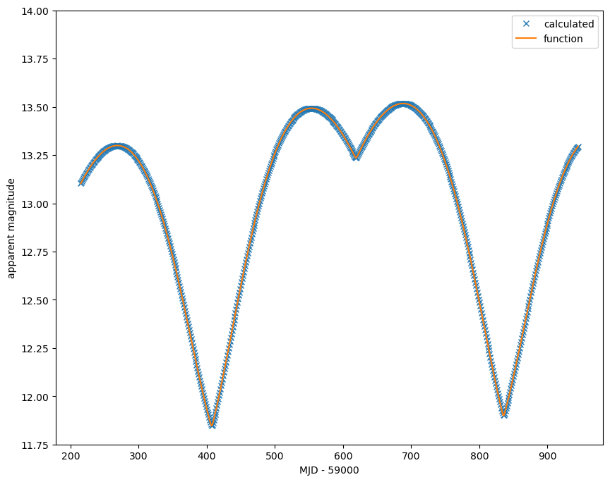
The expected apparent magnitude will thus take the form:

\(m = H + 5 \log_{10}(\Delta) + 5 \log_{10}(r) + S\alpha\)

linear_mag_calc = 5. * np.log10(delta) + 5. * np.log10(r) + H + (S * alpha)

Calculating using the linear phase function model in PPCalculateApparentMagnitudeInFilter…

observations_df = PPCalculateApparentMagnitudeInFilter(observations_df.copy(), 'linear', 'r', 'linear_mag')

fig, ax = plt.subplots(figsize=(10,8))
ax.plot(observations_df["MJD"] - 59000, linear_mag_calc, linestyle="", marker="x", label="calculated")
ax.plot(observations_df["MJD"] - 59000, observations_df["linear_mag"], label="function")
ax.legend()
ax.set_xlabel("MJD - 59000")
ax.set_ylabel("apparent magnitude")
ax.set_ylim((11.75, 14))
plt.show()

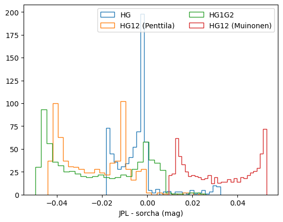
Note that there is some offset (20-40 mmag) between the sorcha predicted magnitudes using the HG/HG12/HG1G2 phase curves and the JPL magnitudes. This is not a bug in sorcha, but rather something in JPL (that is presumably using a more sophisticated model). To show that this is the case, we’ll test these values out using an independent implementation of the three phase curve models.

from scipy.interpolate import CubicSpline

A = [3.332, 1.862]
B = [0.631, 1.218]
C = [0.986, 0.238]

alpha_12 = np.deg2rad([7.5, 30., 60, 90, 120, 150])

phi_1_sp = [7.5e-1, 3.3486016e-1, 1.3410560e-1, 5.1104756e-2, 2.1465687e-2, 3.6396989e-3]
phi_1_derivs = [-1.9098593, -9.1328612e-2]

phi_2_sp = [9.25e-1, 6.2884169e-1, 3.1755495e-1, 1.2716367e-1, 2.2373903e-2, 1.6505689e-4]
phi_2_derivs = [-5.7295780e-1, -8.6573138e-8]

alpha_3 = np.deg2rad([0.0, 0.3, 1., 2., 4., 8., 12., 20., 30.])

phi_3_sp = [1., 8.3381185e-1, 5.7735424e-1, 4.2144772e-1, 2.3174230e-1, 1.0348178e-1, 6.1733473e-2, 1.6107006e-2, 0.]
phi_3_derivs = [-1.0630097, 0]


phi_1 = CubicSpline(alpha_12, phi_1_sp, bc_type=((1,phi_1_derivs[0]),(1,phi_1_derivs[1])))
phi_2 = CubicSpline(alpha_12, phi_2_sp, bc_type=((1,phi_2_derivs[0]),(1,phi_2_derivs[1])))
phi_3 = CubicSpline(alpha_3, phi_3_sp, bc_type=((1,phi_3_derivs[0]),(1,phi_3_derivs[1])))

def HG_model(phase, params):
    sin_a = np.sin(phase)
    tan_ah = np.tan(phase/2)

    W = np.exp(-90.56 * tan_ah * tan_ah)
    scale_sina = sin_a/(0.119 + 1.341*sin_a - 0.754*sin_a*sin_a)

    phi_1_S = 1 - C[0] * scale_sina
    phi_2_S = 1 - C[1] * scale_sina

    phi_1_L = np.exp(-A[0] * np.power(tan_ah, B[0]))
    phi_2_L = np.exp(-A[1] * np.power(tan_ah, B[1]))

    phi_1 = W * phi_1_S + (1-W) * phi_1_L
    phi_2 = W * phi_2_S + (1-W) * phi_2_L
    return params[0] - 2.5*np.log10((1-params[1])* phi_1 + (params[1]) * phi_2)


def HG1G2_model(phase, params):

    tan_ah = np.tan(phase/2)

    phi_1_ev = phi_1(phase)
    phi_2_ev = phi_2(phase)
    phi_3_ev = phi_3(phase)

    msk = phase < 7.5 * np.pi/180

    phi_1_ev[msk] = 1-6*phase[msk]/np.pi
    phi_2_ev[msk] = 1- 9 * phase[msk]/(5*np.pi)

    phi_3_ev[phase > np.pi/6] = 0


    return params[0] - 2.5 * np.log10(params[1] * phi_1_ev + params[2] * phi_2_ev + (1-params[1]-params[2]) * phi_3_ev)

def HG12_model(phase, params):
    if params[1] >= 0.2:
        G1 = +0.9529*params[1] + 0.02162
        G2 = -0.6125*params[1] + 0.5572
    else:
        G1 = +0.7527*params[1] + 0.06164
        G2 = -0.9612*params[1] + 0.6270

    return HG1G2_model(phase, [params[0], G1, G2])

def HG12star_model(phase, params):
    G1 = 0 + params[1] * 0.84293649
    G2 = 0.53513350 - params[1] * 0.53513350

    return HG1G2_model(phase, [params[0], G1, G2])

observations_df['independent_HG'] = observations_df['H_filter'] + 5 * np.log10(observations_df['Range_LTC_km'] * observations_df['Obj_Sun_LTC_km']/(1.495978707e8**2)) + HG_model(observations_df['phase_deg'] * np.pi/180, [0,0.19])
observations_df['independent_HG12'] = observations_df['H_filter'] + 5 * np.log10(observations_df['Range_LTC_km'] * observations_df['Obj_Sun_LTC_km']/(1.495978707e8**2)) + HG12_model(observations_df['phase_deg'] * np.pi/180, [0,0.68])
observations_df['independent_HG12star'] = observations_df['H_filter'] + 5 * np.log10(observations_df['Range_LTC_km'] * observations_df['Obj_Sun_LTC_km']/(1.495978707e8**2)) + HG12star_model(observations_df['phase_deg'] * np.pi/180, [0,0.68])
observations_df['independent_HG1G2'] = observations_df['H_filter'] + 5 * np.log10(observations_df['Range_LTC_km'] * observations_df['Obj_Sun_LTC_km']/(1.495978707e8**2)) + HG1G2_model(observations_df['phase_deg'] * np.pi/180, [0,0.62, 0.14])

plt.hist(observations_df['JPL_mag'] - observations_df['HG_mag'], bins=30, histtype='step', label='HG')
plt.hist(observations_df['JPL_mag'] - observations_df['HG12_mag'], bins=30, histtype='step', label='HG12 (Penttila)')
plt.hist(observations_df['JPL_mag'] - observations_df['HG1G2_mag'], bins=30, histtype='step', label='HG1G2')
plt.hist(observations_df['JPL_mag'] - observations_df['independent_HG12'], bins=30, histtype='step', label='HG12 (Muinonen)')

plt.legend(ncol=2)
plt.xlabel('JPL - sorcha (mag)')
plt.show()


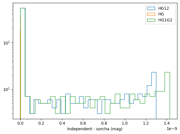
plt.hist(observations_df['HG12_mag'] - observations_df['independent_HG12star'], bins=30, histtype='step', label='HG12')
plt.hist(observations_df['HG_mag'] - observations_df['independent_HG'], bins=30, histtype='step', label='HG')
plt.hist(observations_df['HG1G2_mag'] - observations_df['independent_HG1G2'], bins=30, histtype='step', label='HG1G2 ')
plt.xlabel('Independent - sorcha (mag)')

plt.legend()
plt.tight_layout()
plt.show()

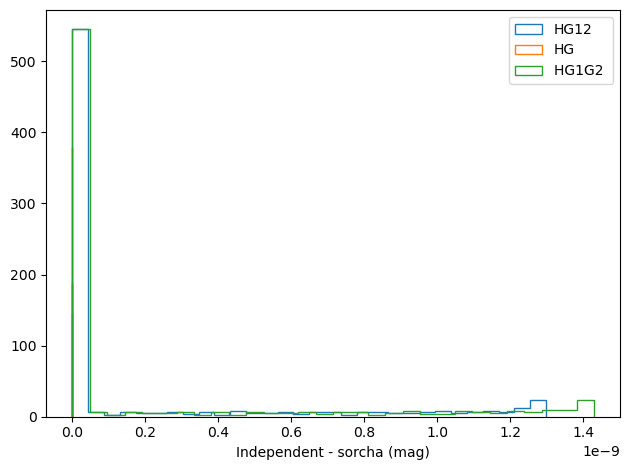
So the differences are \(< 10^{-9}\) between the two implementations.

Let’s look at this plot again with a logarithmic y-axis so you can see the residuals clearer

plt.yscale('log',base=10)
plt.hist(observations_df['HG12_mag'] - observations_df['independent_HG12star'], bins=30, histtype='step', label='HG12')
plt.hist(observations_df['HG_mag'] - observations_df['independent_HG'], bins=30, histtype='step', label='HG')
plt.hist(observations_df['HG1G2_mag'] - observations_df['independent_HG1G2'], bins=30, histtype='step', label='HG1G2 ')
plt.xlabel('Independent - sorcha (mag)')
plt.legend()
plt.tight_layout()
plt.show()