Incorporating lightcurves

The goal of this notebook is to demonstrate the use of lightcurves within sorcha.

This will be done in two different ways:

• We will use the community tools part of the sorcha-addons(https://github.com/dirac-institute/sorcha-addons) package

• We will implement a custom lightcurve, and use it inside the code

The idea is that the user can, in principle, implement their own lightcurves, and incorporate them in their simulation. The goal of sorcha-addons is for both the development team, as well as for the community, to share their implementations of custom lightcurve models.

For more information on creating custom lightcurve models for Sorcha, see (https://sorcha.readthedocs.io/en/latest/postprocessing.html#lightcurve-template-class)

import pandas as pd
import numpy as np
import astropy.units as u
from astroquery.jplhorizons import Horizons
from sorcha_addons.lightcurve.sinusoidal.sinusoidal_lightcurve import SinusoidalLightCurve
from sorcha.modules.PPCalculateApparentMagnitudeInFilter import PPCalculateApparentMagnitudeInFilter
import matplotlib.pyplot as plt

This notebook will not use a realistic set of observations (as in the demo_ApparentMagnitudeValidation notebook), but rather create a toy scenario with a simple to understand and interpret set of results. The general structure of the notebook will be the same.

We will create a dataframe for observations in a similar structure as in the demo_ApparentMagnitudeValidation notebook:

observations_df = pd.DataFrame(
    {
        "fieldMJD_TAI": np.linspace(
            0, 100, 1001
        ),  # time of observation - note these values are bogus, we only care about the Delta t for this demo
        "H_filter": 10 * np.ones(1001),
        "GS": 0.15 * np.ones(1001),
        "G1": 0.62 * np.ones(1001),
        "G2": 0.14 * np.ones(1001),
        "G12": 0.68 * np.ones(1001),
        "S": 0.04 * np.ones(1001),
        "Range_LTC_km": 1.495978707e8 * np.ones(1001),  # 1 au
        "Obj_Sun_LTC_km": 1.495978707e8 * np.ones(1001),  # 1 au
        "phase_deg": np.linspace(0, 10, 1001),
    }
)  # some phase angle variation so we can see the phase curve on top of the lightcurve

observations_df

	fieldMJD_TAI	H_filter	GS	G1	G2	G12	S	Range_LTC_km	Obj_Sun_LTC_km	phase_deg
0	0.0	10.0	0.15	0.62	0.14	0.68	0.04	149597870.7	149597870.7	0.00
1	0.1	10.0	0.15	0.62	0.14	0.68	0.04	149597870.7	149597870.7	0.01
2	0.2	10.0	0.15	0.62	0.14	0.68	0.04	149597870.7	149597870.7	0.02
3	0.3	10.0	0.15	0.62	0.14	0.68	0.04	149597870.7	149597870.7	0.03
4	0.4	10.0	0.15	0.62	0.14	0.68	0.04	149597870.7	149597870.7	0.04
...	...	...	...	...	...	...	...	...	...	...
996	99.6	10.0	0.15	0.62	0.14	0.68	0.04	149597870.7	149597870.7	9.96
997	99.7	10.0	0.15	0.62	0.14	0.68	0.04	149597870.7	149597870.7	9.97
998	99.8	10.0	0.15	0.62	0.14	0.68	0.04	149597870.7	149597870.7	9.98
999	99.9	10.0	0.15	0.62	0.14	0.68	0.04	149597870.7	149597870.7	9.99
1000	100.0	10.0	0.15	0.62	0.14	0.68	0.04	149597870.7	149597870.7	10.00

1001 rows × 10 columns

Now we calculate the magnitude using the various models in PPCalculateApparentMagnitudeInFilter.

observations_df = PPCalculateApparentMagnitudeInFilter(observations_df.copy(), "HG", "r", "HG_mag")
observations_df = PPCalculateApparentMagnitudeInFilter(observations_df.copy(), "HG12", "r", "HG12_mag")
observations_df = PPCalculateApparentMagnitudeInFilter(observations_df.copy(), "HG1G2", "r", "HG1G2_mag")
observations_df = PPCalculateApparentMagnitudeInFilter(observations_df.copy(), "linear", "r", "linear_mag")
observations_df = PPCalculateApparentMagnitudeInFilter(observations_df.copy(), "none", "r", "Simple_mag")

observations_df

	fieldMJD_TAI	H_filter	GS	G1	G2	G12	S	Range_LTC_km	Obj_Sun_LTC_km	phase_deg	HG_mag	HG12_mag	HG1G2_mag	linear_mag	Simple_mag
0	0.0	10.0	0.15	0.62	0.14	0.68	0.04	149597870.7	149597870.7	0.00	10.000000	10.000000	10.000000	10.0000	10.0
1	0.1	10.0	0.15	0.62	0.14	0.68	0.04	149597870.7	149597870.7	0.01	10.001390	10.000361	10.000366	10.0004	10.0
2	0.2	10.0	0.15	0.62	0.14	0.68	0.04	149597870.7	149597870.7	0.02	10.002776	10.000884	10.000884	10.0008	10.0
3	0.3	10.0	0.15	0.62	0.14	0.68	0.04	149597870.7	149597870.7	0.03	10.004158	10.001562	10.001549	10.0012	10.0
4	0.4	10.0	0.15	0.62	0.14	0.68	0.04	149597870.7	149597870.7	0.04	10.005537	10.002388	10.002352	10.0016	10.0
...	...	...	...	...	...	...	...	...	...	...	...	...	...	...	...
996	99.6	10.0	0.15	0.62	0.14	0.68	0.04	149597870.7	149597870.7	9.96	10.656917	10.628635	10.624403	10.3984	10.0
997	99.7	10.0	0.15	0.62	0.14	0.68	0.04	149597870.7	149597870.7	9.97	10.657299	10.629045	10.624827	10.3988	10.0
998	99.8	10.0	0.15	0.62	0.14	0.68	0.04	149597870.7	149597870.7	9.98	10.657681	10.629454	10.625251	10.3992	10.0
999	99.9	10.0	0.15	0.62	0.14	0.68	0.04	149597870.7	149597870.7	9.99	10.658064	10.629864	10.625675	10.3996	10.0
1000	100.0	10.0	0.15	0.62	0.14	0.68	0.04	149597870.7	149597870.7	10.00	10.658445	10.630273	10.626099	10.4000	10.0

1001 rows × 15 columns

Now we can plot the magnitudes and compare them.

fig, ax = plt.subplots(figsize=(10, 8))
ax.plot(observations_df["fieldMJD_TAI"], observations_df["Simple_mag"], linestyle="-", label="No phase curve")
ax.plot(observations_df["fieldMJD_TAI"], observations_df["HG_mag"], label="HG")
ax.plot(observations_df["fieldMJD_TAI"], observations_df["HG12_mag"], label="HG12")
ax.plot(observations_df["fieldMJD_TAI"], observations_df["HG1G2_mag"], label="HG1G2")
ax.plot(observations_df["fieldMJD_TAI"], observations_df["linear_mag"], label="Linear")

ax.legend()
ax.set_xlabel("Time since first observation (days)")
ax.set_ylabel("Apparent magnitude")
plt.gca().invert_yaxis()
plt.grid()
plt.show()

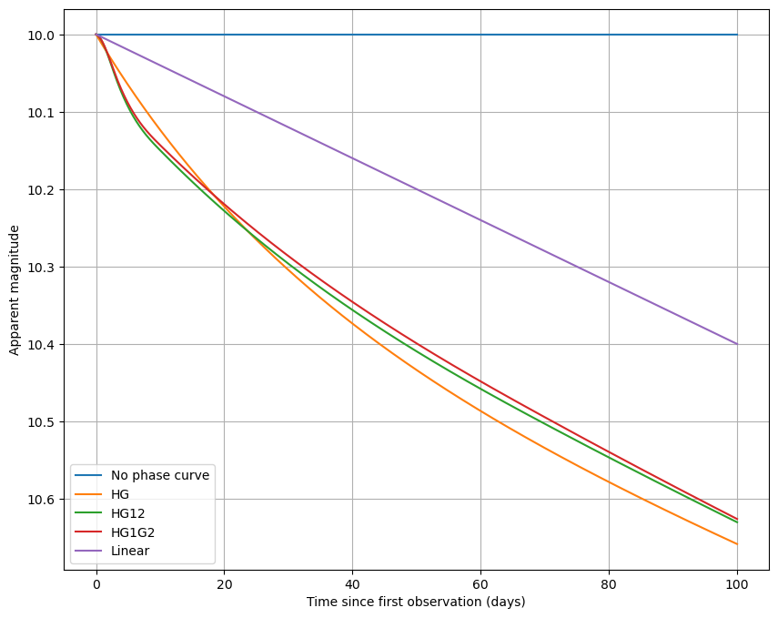
The effect of the lightcurve is to add an extra term to the apparent magnitude, that, in principle, can be a function of the characteristics of the observations, such as time of observation, phase angle or topocentric and heliocentric distances. The entire observational_df dataframe is exposed to the lightcurve, so any dependencies can be added.

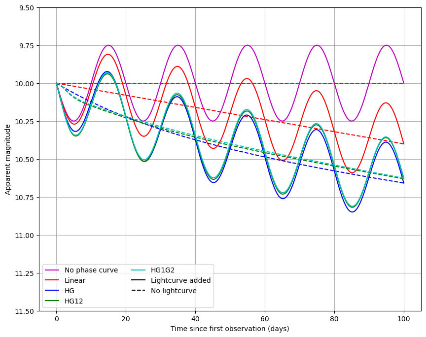
Let’s use the basic sinusoidal lightcurve from sorcha_addons. We need the following columns in our dataframe:

• LCA - lightcurve amplitude [magnitudes].

• Period - period of the sinusoidal oscillation [days]. Should be a positive value.

• Time0 - phase for the light curve [days].

Let’s create a lightcurve with a period of 20 days, phased so that the first observation is at zero variation, and with 0.5 mag peak-to-peak amplitude.

from sorcha.lightcurves.lightcurve_registration import LC_METHODS, update_lc_subclasses

# LC_METHODS is the dictionary that contains all lightcurve implementations
# update_lc_subclasses adds newly defined classes to this dictionary
# this is run by default inside sorcha - we are just showing it here for completeness
update_lc_subclasses()
print(LC_METHODS)

{'identity': <class 'sorcha.lightcurves.identity_lightcurve.IdentityLightCurve'>, 'sinusoidal': <class 'sorcha_addons.lightcurve.sinusoidal.sinusoidal_lightcurve.SinusoidalLightCurve'>}

observations_df["LCA"] = 0.25  # note peak-to-peak is 2LCA!
observations_df["Period"] = 20.0
observations_df["Time0"] = 0.0

observations_df = PPCalculateApparentMagnitudeInFilter(
    observations_df.copy(), "none", "r", "LCA_mag", "sinusoidal"
)
observations_df = PPCalculateApparentMagnitudeInFilter(
    observations_df.copy(), "HG", "r", "LCA_HG_mag", "sinusoidal"
)
observations_df = PPCalculateApparentMagnitudeInFilter(
    observations_df.copy(), "HG12", "r", "LCA_HG12_mag", "sinusoidal"
)
observations_df = PPCalculateApparentMagnitudeInFilter(
    observations_df.copy(), "HG1G2", "r", "LCA_HG1G2_mag", "sinusoidal"
)
observations_df = PPCalculateApparentMagnitudeInFilter(
    observations_df.copy(), "linear", "r", "LCA_linear_mag", "sinusoidal"
)

from matplotlib.lines import Line2D

fig, ax = plt.subplots(figsize=(10, 8))
ax.plot(
    observations_df["fieldMJD_TAI"],
    observations_df["Simple_mag"],
    linestyle="--",
    label="__none__",
    color="m",
)
ax.plot(
    observations_df["fieldMJD_TAI"], observations_df["LCA_mag"], linestyle="-", label="__none__", color="m"
)

ax.plot(
    observations_df["fieldMJD_TAI"],
    observations_df["linear_mag"],
    linestyle="--",
    label="__none__",
    color="r",
)
ax.plot(
    observations_df["fieldMJD_TAI"],
    observations_df["LCA_linear_mag"],
    linestyle="-",
    label="__none__",
    color="r",
)


ax.plot(
    observations_df["fieldMJD_TAI"],
    observations_df["HG_mag"],
    linestyle="--",
    label="__none__",
    color="b",
)
ax.plot(
    observations_df["fieldMJD_TAI"], observations_df["LCA_HG_mag"], linestyle="-", label="__none__", color="b"
)

ax.plot(
    observations_df["fieldMJD_TAI"],
    observations_df["HG12_mag"],
    linestyle="--",
    label="__none__",
    color="g",
)
ax.plot(
    observations_df["fieldMJD_TAI"],
    observations_df["LCA_HG12_mag"],
    linestyle="-",
    label="__none__",
    color="g",
)

ax.plot(
    observations_df["fieldMJD_TAI"],
    observations_df["HG1G2_mag"],
    linestyle="--",
    label="__none__",
    color="c",
)
ax.plot(
    observations_df["fieldMJD_TAI"],
    observations_df["LCA_HG1G2_mag"],
    linestyle="-",
    label="__none__",
    color="c",
)


custom_legend = [
    Line2D([0], [0], color="m", linestyle="-"),
    Line2D([0], [0], color="r", linestyle="-"),
    Line2D([0], [0], color="b", linestyle="-"),
    Line2D([0], [0], color="g", linestyle="-"),
    Line2D([0], [0], color="c", linestyle="-"),
    Line2D([0], [0], color="k", linestyle="-"),
    Line2D([0], [0], color="k", linestyle="--"),
]

ax.legend(
    custom_legend,
    ["No phase curve", "Linear", "HG", "HG12", "HG1G2", "Lightcurve added", "No lightcurve"],
    ncol=2,
)
ax.set_xlabel("Time since first observation (days)")
ax.set_ylabel("Apparent magnitude")
ax.set_ylim(9.5, 11.5)
plt.gca().invert_yaxis()
plt.grid()
plt.show()

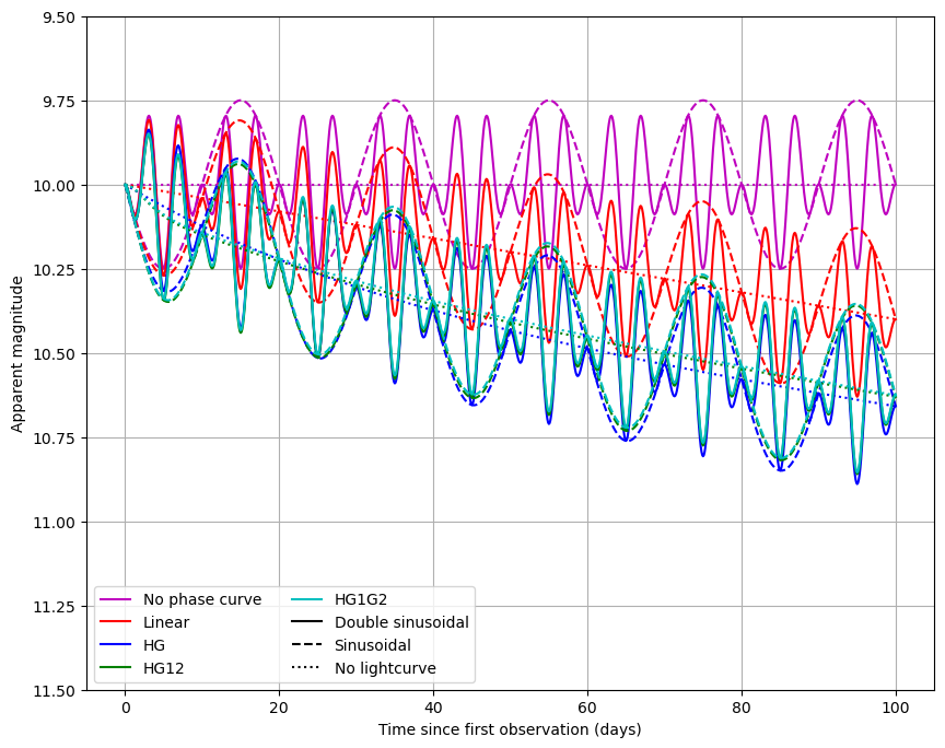
Incorporating your own lightcurve

You can also implement a custom lightcurve. To do so, you need to inherit from the AbstractLightCurve class inside sorcha. Let’s implement a simple extension of this sinusoidal model, where we have two sine terms at once. The implementation will be very similar to the SinusoidalLightCurve class used above.

from sorcha.lightcurves.base_lightcurve import AbstractLightCurve

from sorcha.lightcurves.base_lightcurve import AbstractLightCurve

from typing import List
import pandas as pd
import numpy as np


class DoubleSinusoidalLightCurve(AbstractLightCurve):
    def __init__(
        self, required_column_names: List[str] = ["fieldMJD_TAI", "LCA", "Period1", "Period2", "Time0"]
    ) -> None:
        super().__init__(required_column_names)

    def compute(self, df: pd.DataFrame) -> np.array:
        # Verify that the input data frame contains each of the required columns.
        self._validate_column_names(df)

        time1 = 2 * np.pi * (df["fieldMJD_TAI"] - df["Time0"]) / df["Period1"]
        time2 = 2 * np.pi * (df["fieldMJD_TAI"] - df["Time0"]) / df["Period2"]

        return df["LCA"] * np.sin(time1) * np.sin(time2)

    # this method defines the same of the class inside LC_METHODS
    @staticmethod
    def name_id() -> str:
        return "doublesinusoidal"

update_lc_subclasses()
print(LC_METHODS)

{'identity': <class 'sorcha.lightcurves.identity_lightcurve.IdentityLightCurve'>, 'sinusoidal': <class 'sorcha_addons.lightcurve.sinusoidal.sinusoidal_lightcurve.SinusoidalLightCurve'>, 'doublesinusoidal': <class '__main__.DoubleSinusoidalLightCurve'>}

# let's add the required columns that are different from the sinusoidal lightcurve
observations_df["Period1"] = 20.0
observations_df["Period2"] = 4.0

observations_df = PPCalculateApparentMagnitudeInFilter(
    observations_df.copy(), "none", "r", "DLCA_mag", "doublesinusoidal"
)
observations_df = PPCalculateApparentMagnitudeInFilter(
    observations_df.copy(), "HG", "r", "DLCA_HG_mag", "doublesinusoidal"
)
observations_df = PPCalculateApparentMagnitudeInFilter(
    observations_df.copy(), "HG12", "r", "DLCA_HG12_mag", "doublesinusoidal"
)
observations_df = PPCalculateApparentMagnitudeInFilter(
    observations_df.copy(), "HG1G2", "r", "DLCA_HG1G2_mag", "doublesinusoidal"
)
observations_df = PPCalculateApparentMagnitudeInFilter(
    observations_df.copy(), "linear", "r", "DLCA_linear_mag", "doublesinusoidal"
)

from matplotlib.lines import Line2D

fig, ax = plt.subplots(figsize=(10, 8))
ax.plot(
    observations_df["fieldMJD_TAI"],
    observations_df["Simple_mag"],
    linestyle=":",
    label="__none__",
    color="m",
)
ax.plot(
    observations_df["fieldMJD_TAI"], observations_df["LCA_mag"], linestyle="--", label="__none__", color="m"
)
ax.plot(
    observations_df["fieldMJD_TAI"], observations_df["DLCA_mag"], linestyle="-", label="__none__", color="m"
)


ax.plot(
    observations_df["fieldMJD_TAI"],
    observations_df["linear_mag"],
    linestyle=":",
    label="__none__",
    color="r",
)
ax.plot(
    observations_df["fieldMJD_TAI"],
    observations_df["LCA_linear_mag"],
    linestyle="--",
    label="__none__",
    color="r",
)
ax.plot(
    observations_df["fieldMJD_TAI"],
    observations_df["DLCA_linear_mag"],
    linestyle="-",
    label="__none__",
    color="r",
)


ax.plot(
    observations_df["fieldMJD_TAI"],
    observations_df["HG_mag"],
    linestyle=":",
    label="__none__",
    color="b",
)
ax.plot(
    observations_df["fieldMJD_TAI"],
    observations_df["LCA_HG_mag"],
    linestyle="--",
    label="__none__",
    color="b",
)
ax.plot(
    observations_df["fieldMJD_TAI"],
    observations_df["DLCA_HG_mag"],
    linestyle="-",
    label="__none__",
    color="b",
)

ax.plot(
    observations_df["fieldMJD_TAI"],
    observations_df["HG12_mag"],
    linestyle=":",
    label="__none__",
    color="g",
)
ax.plot(
    observations_df["fieldMJD_TAI"],
    observations_df["LCA_HG12_mag"],
    linestyle="--",
    label="__none__",
    color="g",
)
ax.plot(
    observations_df["fieldMJD_TAI"],
    observations_df["DLCA_HG12_mag"],
    linestyle="-",
    label="__none__",
    color="g",
)

ax.plot(
    observations_df["fieldMJD_TAI"],
    observations_df["HG1G2_mag"],
    linestyle=":",
    label="__none__",
    color="c",
)
ax.plot(
    observations_df["fieldMJD_TAI"],
    observations_df["LCA_HG1G2_mag"],
    linestyle="--",
    label="__none__",
    color="c",
)
ax.plot(
    observations_df["fieldMJD_TAI"],
    observations_df["DLCA_HG1G2_mag"],
    linestyle="-",
    label="__none__",
    color="c",
)


custom_legend = [
    Line2D([0], [0], color="m", linestyle="-"),
    Line2D([0], [0], color="r", linestyle="-"),
    Line2D([0], [0], color="b", linestyle="-"),
    Line2D([0], [0], color="g", linestyle="-"),
    Line2D([0], [0], color="c", linestyle="-"),
    Line2D([0], [0], color="k", linestyle="-"),
    Line2D([0], [0], color="k", linestyle="--"),
    Line2D([0], [0], color="k", linestyle=":"),
]

ax.legend(
    custom_legend,
    ["No phase curve", "Linear", "HG", "HG12", "HG1G2", "Double sinusoidal", "Sinusoidal", "No lightcurve"],
    ncol=2,
)
ax.set_xlabel("Time since first observation (days)")
ax.set_ylabel("Apparent magnitude")
ax.set_ylim(9.5, 11.5)
plt.gca().invert_yaxis()
plt.grid()
plt.show()