Incorporating Cometary Activity

The goal of this notebook is to demonstrate the apply cometary activity within Sorcha.

We will use the community tools part of the Sorcha-addons(https://github.com/dirac-institute/sorcha-addons) package

The idea is that the user can, in principle, implement their own method for cometary activity, and incorporate it in their simulation. The goal of Sorcha-addons is for both the development team, as well as for the community, to share their implementations of custom cometary activity models.

For more information on creating custom comet activity models for Sorcha, see (https://sorcha.readthedocs.io/en/latest/postprocessing.html#cometary-activity-template-class)

import pandas as pd
import numpy as np
import astropy.units as u
import matplotlib.pyplot as plt
from sorcha.modules.PPCalculateApparentMagnitudeInFilter import PPCalculateApparentMagnitudeInFilter
from matplotlib.lines import Line2D
plt.rcParams.update({'font.size': 14})

This notebook will not use a realistic set of observations (as in the demo_ApparentMagnitudeValidation notebook), but rather create a toy scenario with a simple to understand and interpret set of results.

We will create a dataframe for observations in a similar structure as in the demo_ApparentMagnitudeValidation notebook:

observations_df = pd.DataFrame(
    {
        "fieldMJD_TAI": np.linspace(
            0, 100, 1001
        ),  # time of observation - note these values are bogus, we only care about the Delta t for this demo
        "H_filter": 17 * np.ones(1001),
        # starting at 30 au and coming inward to 5 au
        "Range_LTC_km": 1.495978707e8 * np.flip(np.linspace(  0.2, 30, 1001)), # au
        "Obj_Sun_LTC_km": 1.495978707e8 * np.flip(np.linspace(1.2, 30, 1001)),  #  au
        "phase_deg": np.zeros(1001),
        #keeping the same phase although this is unphysical so that we can look at just the effects of activity on the brightness of the object
        "optFilter": np.full(1001,'r',dtype=str),
    }
)

observations_df

	fieldMJD_TAI	H_filter	Range_LTC_km	Obj_Sun_LTC_km	phase_deg	optFilter
0	0.0	17.0	4.487936e+09	4.487936e+09	0.0	r
1	0.1	17.0	4.483478e+09	4.483628e+09	0.0	r
2	0.2	17.0	4.479020e+09	4.479319e+09	0.0	r
3	0.3	17.0	4.474562e+09	4.475011e+09	0.0	r
4	0.4	17.0	4.470104e+09	4.470702e+09	0.0	r
...	...	...	...	...	...	...
996	99.6	17.0	4.775164e+07	1.967511e+08	0.0	r
997	99.7	17.0	4.329362e+07	1.924427e+08	0.0	r
998	99.8	17.0	3.883561e+07	1.881343e+08	0.0	r
999	99.9	17.0	3.437759e+07	1.838259e+08	0.0	r
1000	100.0	17.0	2.991957e+07	1.795174e+08	0.0	r

1001 rows × 6 columns

Now we calculate the magnitude of the nucleus assuming no phase curve model in PPCalculateApparentMagnitudeInFilter.

observations_df = PPCalculateApparentMagnitudeInFilter(observations_df.copy(), "none", "r", "Simple_mag")

observations_df

	fieldMJD_TAI	H_filter	Range_LTC_km	Obj_Sun_LTC_km	phase_deg	optFilter	Simple_mag
0	0.0	17.0	4.487936e+09	4.487936e+09	0.0	r	31.771213
1	0.1	17.0	4.483478e+09	4.483628e+09	0.0	r	31.766969
2	0.2	17.0	4.479020e+09	4.479319e+09	0.0	r	31.762721
3	0.3	17.0	4.474562e+09	4.475011e+09	0.0	r	31.758469
4	0.4	17.0	4.470104e+09	4.470702e+09	0.0	r	31.754213
...	...	...	...	...	...	...	...
996	99.6	17.0	4.775164e+07	1.967511e+08	0.0	r	15.115273
997	99.7	17.0	4.329362e+07	1.924427e+08	0.0	r	14.854373
998	99.8	17.0	3.883561e+07	1.881343e+08	0.0	r	14.569236
999	99.9	17.0	3.437759e+07	1.838259e+08	0.0	r	14.254156
1000	100.0	17.0	2.991957e+07	1.795174e+08	0.0	r	13.901056

1001 rows × 7 columns

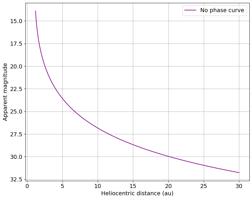
Now we can plot the apparent magnitude of the inactive comet nucleus over time assuming no phase curve effects. Only the changing heliocentric and geocentric distances matter here.

fig, ax = plt.subplots(figsize=(10, 8))
ax.plot(observations_df["fieldMJD_TAI"], observations_df["Simple_mag"], linestyle="-", label="No phase curve")

ax.legend()
ax.set_xlabel("Time since first observation (days)")
ax.set_ylabel("Apparent magnitude")
plt.gca().invert_yaxis()
plt.grid()
plt.show()

fig, ax = plt.subplots(figsize=(10, 8))
ax.plot(observations_df["Obj_Sun_LTC_km"]/1.495978707e8 , observations_df["Simple_mag"], linestyle="-", label="No phase curve", color='purple')

ax.legend()
ax.set_ylabel("Apparent magnitude")
ax.set_xlabel("Heliocentric distance (au)")
plt.gca().invert_yaxis()
plt.grid()
plt.show()

The effect of the cometary activity class is compute the apparent magnitude of the active object from an input apparent magnitude of the nucleus. The entire observational_df dataframe is exposed to the cometary activty class, so any dependencies can be added.

Let’s use the LSSTCometActivity class from sorcha_addons. We need the following columns in our dataframe:

• afrho1 = V-band Afρ value of the comet at 1 au [cm]

• k = power-law slope that describes how the activity varies with heliocentric distance

Let’s activate the LSSTCometActivity class

from sorcha_addons.activity.lsst_comet.lsst_comet_activity import LSSTCometActivity
from sorcha.activity.activity_registration import update_activity_subclasses

update_activity_subclasses()

Let’s calculate the apparent magnitude assuming

observations_df["afrho1"] = 150
observations_df["k"] =-0.3

observations_df = PPCalculateApparentMagnitudeInFilter(observations_df.copy(), "none", "r",cometary_activity_choice="lsst_comet")

observations_df

	fieldMJD_TAI	H_filter	Range_LTC_km	Obj_Sun_LTC_km	phase_deg	optFilter	Simple_mag	afrho1	k	trailedSourceMagTrue	coma_magnitude
0	0.0	17.0	4.487936e+09	4.487936e+09	0.0	r	31.771213	150	-0.3	27.523035	27.544954
1	0.1	17.0	4.483478e+09	4.483628e+09	0.0	r	31.766969	150	-0.3	27.519542	27.541477
2	0.2	17.0	4.479020e+09	4.479319e+09	0.0	r	31.762721	150	-0.3	27.516046	27.537996
3	0.3	17.0	4.474562e+09	4.475011e+09	0.0	r	31.758469	150	-0.3	27.512546	27.534512
4	0.4	17.0	4.470104e+09	4.470702e+09	0.0	r	31.754213	150	-0.3	27.509043	27.531024
...	...	...	...	...	...	...	...	...	...	...	...
996	99.6	17.0	4.775164e+07	1.967511e+08	0.0	r	15.115273	150	-0.3	14.195410	14.803064
997	99.7	17.0	4.329362e+07	1.924427e+08	0.0	r	14.854373	150	-0.3	13.990077	14.641362
998	99.8	17.0	3.883561e+07	1.881343e+08	0.0	r	14.569236	150	-0.3	13.764254	14.466835
999	99.9	17.0	3.437759e+07	1.838259e+08	0.0	r	14.254156	150	-0.3	13.512743	14.276596
1000	100.0	17.0	2.991957e+07	1.795174e+08	0.0	r	13.901056	150	-0.3	13.228088	14.066571

1001 rows × 11 columns

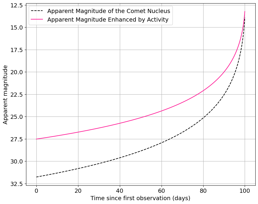
Let’s plot by time

fig, ax = plt.subplots(figsize=(10, 8))
ax.plot(
    observations_df["fieldMJD_TAI"],
    observations_df["Simple_mag"],
    linestyle="--",
    label="Apparent Magnitude of the Comet Nucleus",
    color="black",
)
ax.plot(
    observations_df["fieldMJD_TAI"], observations_df["trailedSourceMagTrue"], linestyle="-", label="Apparent Magnitude Enhanced by Activity", color="deeppink"
)

plt.legend()
ax.set_xlabel("Time since first observation (days)")
ax.set_ylabel("Apparent magnitude")
plt.gca().invert_yaxis()
plt.grid()
plt.show()

Let’s plot by time and look closer to perihleion

fig, ax = plt.subplots(figsize=(10, 8))
ax.plot(
    observations_df["fieldMJD_TAI"],
    observations_df["Simple_mag"],
    linestyle="--",
    label="Apparent Magnitude of the Comet Nucleus",
    color="black",
)
ax.plot(
    observations_df["fieldMJD_TAI"], observations_df["trailedSourceMagTrue"], linestyle="-", label="Apparent Magnitude Enhanced by Activity", color="deeppink"
)

plt.legend()
ax.set_xlabel("Time since first observation (days)")
ax.set_ylabel("Apparent magnitude")
plt.gca().invert_yaxis()
plt.xlim(80,100)
plt.grid()
plt.show()

Let’s plot by heliocentric distance

fig, ax = plt.subplots(figsize=(10, 8))
ax.plot(
    observations_df["Obj_Sun_LTC_km"]/1.495978707e8,
    observations_df["Simple_mag"],
    linestyle="--",
    label="Apparent Magnitude of the Comet Nucleus",
    color="black",
)
ax.plot(
    observations_df["Obj_Sun_LTC_km"]/1.495978707e8, observations_df["trailedSourceMagTrue"], linestyle="-", label="Apparent Magnitude Enhanced by Activity", color="deeppink"
)

plt.legend()
ax.set_xlabel("Heliocentric distance (au)")
ax.set_ylabel("Apparent magnitude")
plt.gca().invert_yaxis()
plt.grid()
plt.show()

Let’s plot by heliocentric distance and zoom in close to perihelion

fig, ax = plt.subplots(figsize=(10, 8))
ax.plot(
    observations_df["Obj_Sun_LTC_km"]/1.495978707e8,
    observations_df["Simple_mag"],
    linestyle="--",
    label="Apparent Magnitude of the Comet Nucleus",
    color="black",
)
ax.plot(
    observations_df["Obj_Sun_LTC_km"]/1.495978707e8, observations_df["trailedSourceMagTrue"], linestyle="-", label="Apparent Magnitude Enhanced by Activity", color="deeppink"
)

plt.legend()
ax.set_xlabel("Heliocentric distance (au)")
ax.set_ylabel("Apparent magnitude")
plt.gca().invert_yaxis()
plt.xlim(1.0,2)
plt.grid()
plt.show()

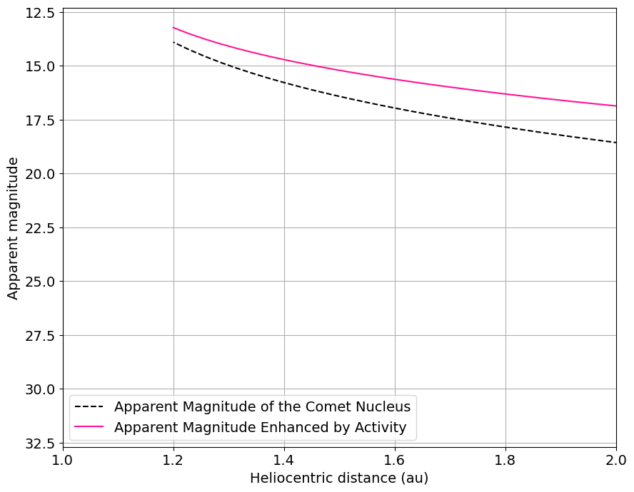
At larger heliocentric distances the nucelus does not contribute much. The coma is the main contribution to the apparent magnitude at those distances, and the comet is observed to be much brighter than an inactive body at the same heliocentric distance. Closer to the Sun, the nucleus contribution to the apparent magntiude is more significant.