Detection Efficiency Filter Demo

This notebook demonstrates the detection efficiency/fading function filter. The equation for the fading function is taken from Veres & Chesley (2017):

\[\epsilon(m) = \frac{F}{1 + e^\frac{m-m_{5\sigma}}{w}}\]

where \(\epsilon(m)\) is the probability of detection, \(F\) is the peak detection efficiency, \(m\) and \(m_{5\sigma}\) are respectively the observed magnitude and \(5\sigma\) limiting magnitude of the pointing, and \(w\) is the width of the fading function.

from sorcha.modules.PPFadingFunctionFilter import PPFadingFunctionFilter
from sorcha.utilities.sorchaModuleRNG import PerModuleRNG

import pandas as pd
import matplotlib.pyplot as plt
import numpy as np

Create a dataframe of synthetic observations

Only the apparent magnitude and the five-sigma limiting depth are needed for this. For simplicity, we will set the five-sigma limiting depth to be constant for all observations.

nobs_per_field = 1000000

mags = np.random.uniform(23.0, 26.0, nobs_per_field)
five_sigma = np.zeros(nobs_per_field) + 24.5
random_obs = pd.DataFrame({"PSFMag":mags, "fiveSigmaDepth_mag":five_sigma})

random_obs

	PSFMag	fiveSigmaDepth_mag
0	23.714230	24.5
1	25.921639	24.5
2	24.809060	24.5
3	24.450894	24.5
4	24.829012	24.5
...	...	...
999995	24.655972	24.5
999996	25.373721	24.5
999997	25.008599	24.5
999998	23.506419	24.5
999999	23.894184	24.5

1000000 rows × 2 columns

We can apply the fading function filter implementation in Sorcha to the randomised observations.

peak_efficiency = 1.0
width = 0.1
rng=PerModuleRNG(2021)
reduced_obs = PPFadingFunctionFilter(random_obs, peak_efficiency, width, rng)

Now we calculate the probabilty of each observation to survive Sorcha’s fading function filter, binned by magnitude.

bin_width = 0.04
magbins = np.arange(23.0, 26.0, bin_width)

magcounts, _ = np.histogram(random_obs['PSFMag'].values, bins=magbins)

redmagcounts, _ = np.histogram(reduced_obs['PSFMag'].values, bins=magbins)

sorcha_probability = redmagcounts/magcounts

And we can compare this to the calculated detection probability of each magnitude bin, using Equation One.

calculated_probability = peak_efficiency / (1.0 + np.exp((magbins - 24.5) / width))

fig, ax = plt.subplots(1, figsize=(8, 6))
ax.bar(magbins[:-1], sorcha_probability, align="edge", width=bin_width, color="mediumaquamarine", label="Sorcha detection probability")
ax.set_ylim((0, 1.1))
ax.set_xlim((23, 26))
ax.set_xlabel("PSF magnitude")
ax.set_ylabel("detection probability")
ax.plot(magbins, calculated_probability, color="darkslateblue", label="calculated detection probability")
ax.legend()
plt.show()

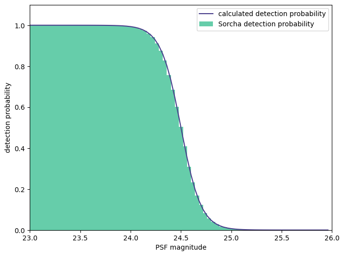
Sorcha’s detection probability clearly follows the expected curve.

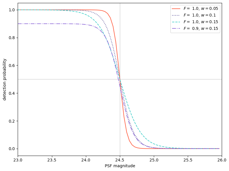
We can also take a look at how the fading function/detection efficiency changes with parameters.

def deteff(mags, fivesig, peak, width):
    return peak / (1.0 + np.exp((mags - fivesig) / width))

colors = plt.get_cmap('gnuplot', 3)
x = colors(np.arange(0,3,1))

widths = [0.05, 0.1, 0.15]
colors = ["tomato", "darkslateblue", "mediumturquoise"]
styles = ["solid", "dotted", "dashed"]

fig, ax = plt.subplots(1, figsize=(8, 6))

ax.axvline(24.5, 0, 1, linestyle="-", alpha=0.5, color="grey", linewidth=0.8)
ax.axhline(0.5, 0, 1, linestyle="-", alpha=0.5, color="grey", linewidth=0.8)

for i, width in enumerate(widths):
    y = deteff(magbins, 24.5, 1., width)
    ax.plot(magbins, y, color=colors[i], linestyle=styles[i], label=f"$F = $ 1.0, $w = {width}$")

y = deteff(magbins, 24.5, .9, 0.1)
ax.plot(magbins, y, color="mediumpurple", linestyle="dashdot", label=f"$F = $ 0.9, $w = {width}$")

ax.set_xlim((23, 26))
ax.legend()
ax.set_xlabel("PSF magnitude")
ax.set_ylabel("detection probability")

fig.tight_layout()
plt.show()