Uncertainties and Randomization Demo

[1]:

from sorcha.modules.PPAddUncertainties import addUncertainties
from sorcha.modules.PPRandomizeMeasurements import randomizeAstrometryAndPhotometry, randomizeAstrometry
from sorcha.utilities.sorchaModuleRNG import PerModuleRNG

[2]:

import numpy as np
import pandas as pd
import matplotlib.pyplot as plt
from astropy.coordinates import SkyCoord
from sorcha.utilities.sorchaConfigs import expertConfigs

This notebook demonstrates the uncertainties calculation and the randomisation of object position and magnitude based on the calculated uncertainties.

First we create the data. The expected LSST limiting magnitude for a single exposure in the g-band is 25 - we will extend our magnitude range to 30 for demonstrative purposes. The objects have identical position, velocity, seeing and limiting magnitude at the source position: uncertainties will thus depend on magnitude alone.

[3]:

obj_ids = np.arange(0, 1000)
obj_mags = np.linspace(15, 30, 1000)
psf_mags = obj_mags + 0.01
sig_limit = np.ones(len(obj_ids)) + 23.
seeing = np.ones(len(obj_ids))
astRArate = np.ones(len(obj_ids)) + 0.03
astDecrate = np.ones(len(obj_ids)) - 0.01
astRA = np.ones(len(obj_ids)) + 260.
astDec = np.ones(len(obj_ids)) -5.
texp = np.ones(len(obj_ids)) * 30.0

[4]:

observations = pd.DataFrame({'ObjID': obj_ids,
                             'trailedSourceMagTrue': obj_mags,
                             'PSFMagTrue': psf_mags,
                             'fiveSigmaDepth_mag': sig_limit,
                             'seeingFwhmGeom_arcsec': seeing,
                             'RARateCosDec_deg_day': astRArate,
                             'DecRate_deg_day': astDecrate,
                             'RA_deg': astRA,
                             'Dec_deg': astDec,
                             'visitExposureTime': texp,
                             })

[5]:

observations.columns

[5]:

Index(['ObjID', 'trailedSourceMagTrue', 'PSFMagTrue', 'fiveSigmaDepth_mag',
       'seeingFwhmGeom_arcsec', 'RARateCosDec_deg_day', 'DecRate_deg_day',
       'RA_deg', 'Dec_deg', 'visitExposureTime'],
      dtype='object')

As can be seen from the columns, both trailedSourceMagTrue (the magnitude of the source including any trailing) and PSFMagTrue (the magnitude of the object within the PSF-fitting kernel) are included here. The code will calculate the uncertainties for each one.

[6]:

configs = {'trailing_losses_on':True, 'default_snr_cut': False}
configs = expertConfigs(**configs)
setattr(configs, "expert", configs)
rng = PerModuleRNG(2012)

[7]:

obs_uncert_1 = addUncertainties(observations, configs, rng)
obs_uncert = randomizeAstrometryAndPhotometry(obs_uncert_1, configs, rng)

[8]:

obs_uncert.columns

[8]:

Index(['ObjID', 'trailedSourceMagTrue', 'PSFMagTrue', 'fiveSigmaDepth_mag',
       'seeingFwhmGeom_arcsec', 'RARateCosDec_deg_day', 'DecRate_deg_day',
       'RATrue_deg', 'DecTrue_deg', 'visitExposureTime',
       'astrometricSigma_deg', 'trailedSourceMagSigma', 'SNR', 'PSFMagSigma',
       'trailedSourceMag', 'PSFMag', 'RA_deg', 'Dec_deg'],
      dtype='object')

[9]:

obs_uncert

[9]:

	ObjID	trailedSourceMagTrue	PSFMagTrue	fiveSigmaDepth_mag	seeingFwhmGeom_arcsec	RARateCosDec_deg_day	DecRate_deg_day	RATrue_deg	DecTrue_deg	visitExposureTime	astrometricSigma_deg	trailedSourceMagSigma	SNR	PSFMagSigma	trailedSourceMag	PSFMag	RA_deg	Dec_deg
0	0	15.000000	15.010000	24.0	1.0	1.03	0.99	261.0	-4.0	30.0	0.000003	0.000677	1595.148457	0.000680	15.000116	15.009979	261.000001	-4.000001
1	1	15.015015	15.025015	24.0	1.0	1.03	0.99	261.0	-4.0	30.0	0.000003	0.000682	1583.992536	0.000685	15.015128	15.025376	261.000001	-3.999998
2	2	15.030030	15.040030	24.0	1.0	1.03	0.99	261.0	-4.0	30.0	0.000003	0.000687	1572.912403	0.000690	15.030911	15.039235	260.999999	-4.000004
3	3	15.045045	15.055045	24.0	1.0	1.03	0.99	261.0	-4.0	30.0	0.000003	0.000692	1561.907528	0.000695	15.045742	15.056046	260.999996	-4.000001
4	4	15.060060	15.070060	24.0	1.0	1.03	0.99	261.0	-4.0	30.0	0.000003	0.000697	1550.977385	0.000700	15.059227	15.070627	260.999997	-4.000005
...	...	...	...	...	...	...	...	...	...	...	...	...	...	...	...	...	...	...
995	995	29.939940	29.949940	24.0	1.0	1.03	0.99	261.0	-4.0	30.0	0.011947	4.653574	0.013823	4.663437	29.850508	33.209062	261.003245	-4.001115
996	996	29.954955	29.964955	24.0	1.0	1.03	0.99	261.0	-4.0	30.0	0.012113	4.668383	0.013633	4.678248	24.605097	27.878347	260.996668	-4.005759
997	997	29.969970	29.979970	24.0	1.0	1.03	0.99	261.0	-4.0	30.0	0.012282	4.683196	0.013445	4.693062	37.811662	31.596631	261.010172	-4.009016
998	998	29.984985	29.994985	24.0	1.0	1.03	0.99	261.0	-4.0	30.0	0.012453	4.698010	0.013261	4.707879	31.139893	23.026854	260.982451	-4.021063
999	999	30.000000	30.010000	24.0	1.0	1.03	0.99	261.0	-4.0	30.0	0.012627	4.712828	0.013079	4.722698	34.986386	29.345251	260.981810	-4.001609

1000 rows × 18 columns

As can be seen from the above, we have several new columns:

trailedSourceMag/PSFMag: a randomised magnitude as observed by the telescope, based on the ‘true’ magnitude and its calculated uncertainty

trailedSourceMagSigma/PSFMagSigma: the uncertainty on the magnitude measurement

astrometricSigma_deg: the uncertainty on the object position

SNR: the signal-to-noise ratio.

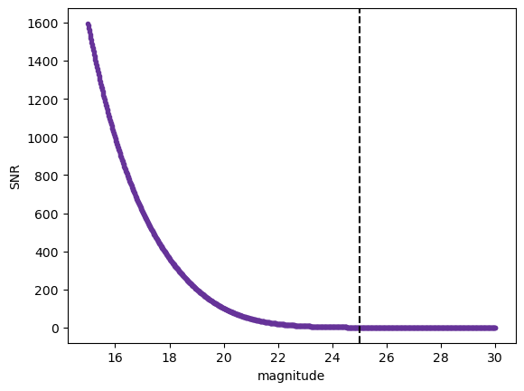
Let’s take a look at these, starting with the SNR. For all plots, the single-exposure limiting magnitude in g-band (25) is marked.

[10]:

fig, ax = plt.subplots(1)
ax.plot(obs_uncert['trailedSourceMagTrue'].values, obs_uncert['SNR'].values, linestyle='', marker='.', color='rebeccapurple')
ax.axvline(25, color='black', linestyle='--')
ax.set_xlabel('magnitude')
ax.set_ylabel('SNR')
plt.show()

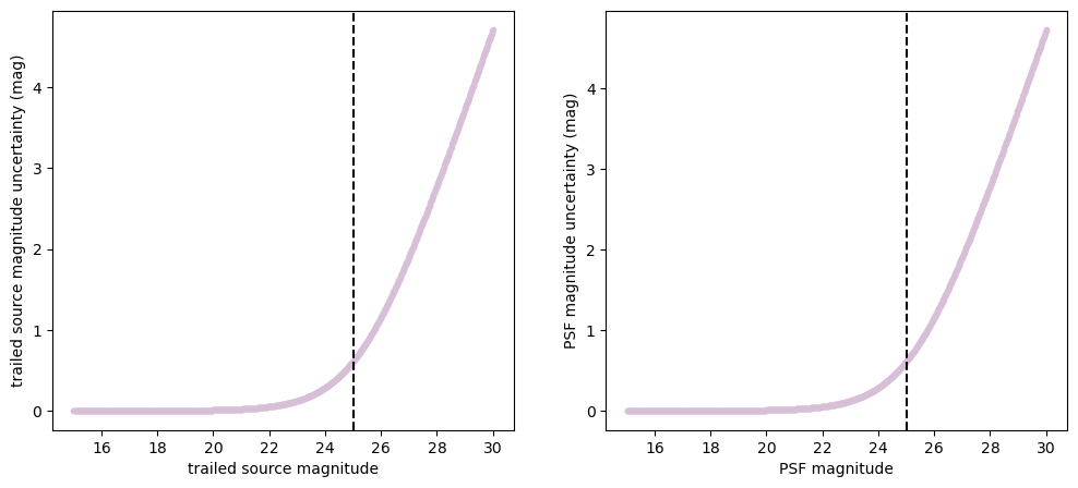
../_images/notebooks_demo_UncertaintiesAndRandomization_13_0.png

The photometric uncertainty for the trailed source and PSF magnitudes:

[11]:

fig, ax = plt.subplots(1, 2, figsize=(12, 5))
ax[0].plot(obs_uncert['trailedSourceMagTrue'].values, obs_uncert['trailedSourceMagSigma'].values, linestyle='', marker='.', color='thistle')
ax[0].set_xlabel('trailed source magnitude')
ax[0].set_ylabel('trailed source magnitude uncertainty (mag)')
ax[0].axvline(25, color='black', linestyle='--')
ax[1].plot(obs_uncert['PSFMagTrue'].values, obs_uncert['PSFMagSigma'].values, linestyle='', marker='.', color='thistle')
ax[1].set_xlabel('PSF magnitude')
ax[1].set_ylabel('PSF magnitude uncertainty (mag)')
ax[1].axvline(25, color='black', linestyle='--')
plt.show()

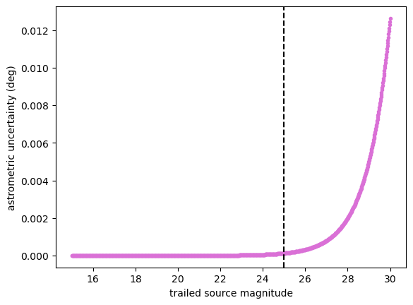
../_images/notebooks_demo_UncertaintiesAndRandomization_15_0.png

Astrometric uncertainty:

[12]:

fig, ax = plt.subplots(1)
ax.plot(obs_uncert['trailedSourceMagTrue'].values, obs_uncert['astrometricSigma_deg'].values, linestyle='', marker='.', color='orchid')
ax.axvline(25, color='black', linestyle='--')
ax.set_xlabel('trailed source magnitude')
ax.set_ylabel('astrometric uncertainty (deg)')
plt.show()

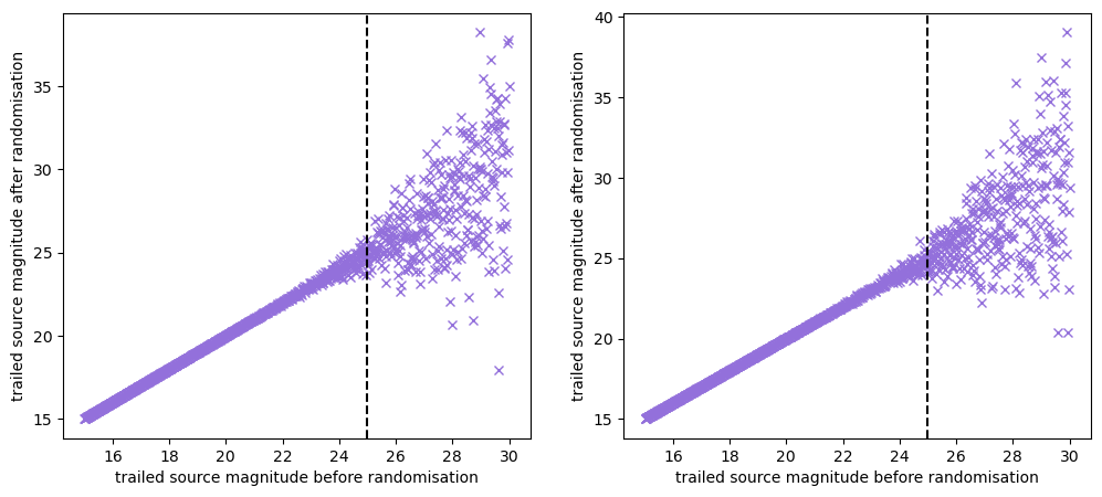
../_images/notebooks_demo_UncertaintiesAndRandomization_17_0.png

Next we look at the randomisation of the magnitude based on the uncertainties, for both trailed source and PSF magnitudes. Note that for large magnitudes, and thus large photometric uncertainties, the randomisation leads to very large shifts in the magnitude. However, this only occurs for objects fainter than LSST’s single exposure limiting magnitude - the SNR of these objects is so low that by default, SSPP will remove them from contention.

[13]:

fig, ax = plt.subplots(1, 2, figsize=(12, 5))
ax[0].plot(obs_uncert['trailedSourceMagTrue'].values, obs_uncert['trailedSourceMag'].values, linestyle="", marker="x", color='mediumpurple')
ax[0].set_xlabel('trailed source magnitude before randomisation')
ax[0].set_ylabel('trailed source magnitude after randomisation')
ax[0].axvline(25, color='black', linestyle='--')
ax[1].plot(obs_uncert['PSFMagTrue'].values, obs_uncert['PSFMag'].values, linestyle="", marker="x", color='mediumpurple')
ax[1].set_xlabel('trailed source magnitude before randomisation')
ax[1].set_ylabel('trailed source magnitude after randomisation')
ax[1].axvline(25, color='black', linestyle='--')
plt.show()

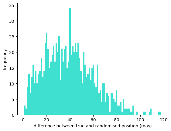
../_images/notebooks_demo_UncertaintiesAndRandomization_19_0.png

A separate function then randomises the object position based on its astrometric uncertainty. We will recreate the data to have the same magnitude, but vary RA and Dec.

[14]:

obj_ids = np.arange(0, 1000)
obj_mags = np.ones(len(obj_ids)) + 21.
psf_mags = obj_mags + 0.01
sig_limit = np.ones(len(obj_ids)) + 23.
seeing = np.ones(len(obj_ids))
astRArate = np.ones(len(obj_ids)) + 0.03
astDecrate = np.ones(len(obj_ids)) - 0.01
astRA = np.linspace(0, 360, 1000)
astDec = np.linspace(-90, 0, 1000)
texp = np.ones(len(obj_ids)) * 30.0

[15]:

observations = pd.DataFrame({'ObjID': obj_ids,
                             'trailedSourceMagTrue': obj_mags,
                             'PSFMagTrue': psf_mags,
                             'fiveSigmaDepth_mag': sig_limit,
                             'seeingFwhmGeom_arcsec': seeing,
                             'RARateCosDec_deg_day': astRArate,
                             'DecRate_deg_day': astDecrate,
                             'RA_deg': astRA,
                             'Dec_deg': astDec,
                             'visitExposureTime': texp,
                             })

[16]:

observations = addUncertainties(observations, configs, rng)

[17]:

observations = randomizeAstrometry(observations, rng, sigName='astrometricSigma_deg', sigUnits='deg')

[18]:

true_coord = SkyCoord(ra=observations['RATrue_deg'].values, dec=observations['DecTrue_deg'].values, unit="deg")
random_coord = SkyCoord(ra=observations['RA_deg'].values, dec=observations['Dec_deg'].values, unit="deg")

separation = true_coord.separation(random_coord).mas

[19]:

fig, ax = plt.subplots(1)
ax.hist(separation, 100, color='turquoise')
ax.set_ylabel('frequency')
ax.set_xlabel('difference between true and randomised position (mas)')
plt.show()

../_images/notebooks_demo_UncertaintiesAndRandomization_26_0.png